Repository of Reproducible Computations

Free Statistics

of Irreproducible Research!

Author's title

Author

*The author of this computation has been verified*

R Software Module

rwasp_edauni.wasp

Title produced by software

Univariate Explorative Data Analysis

Date of computation

Wed, 04 Nov 2009 09:38:24 -0700

Cite this page as follows

Statistical Computations at FreeStatistics.org, Office for Research Development and Education, URL https://freestatistics.org/blog/index.php?v=date/2009/Nov/04/t1257352751os8mx1ucdahjrzm.htm/, Retrieved Mon, 29 Apr 2024 10:00:00 +0000

Statistical Computations at FreeStatistics.org, Office for Research Development and Education, URL https://freestatistics.org/blog/index.php?pk=53703, Retrieved Mon, 29 Apr 2024 10:00:00 +0000

QR Codes:

Paste this QR Code to cite your computation.

Original text written by user:

IsPrivate?

No (this computation is public)

User-defined keywords

Estimated Impact

109

Family? (F = Feedback message, R = changed R code, M = changed R Module, P = changed Parameters, D = changed Data)

-       [Univariate Explorative Data Analysis] [Ws 5 univariate E...] [2009-11-04 16:38:24] [ba02bcb7e07025bbb7f8a074d38ad767] [Current]
-    D    [Univariate Explorative Data Analysis] [Ws 5] [2009-11-05 10:51:20] [74be16979710d4c4e7c6647856088456] 
-    D      [Univariate Explorative Data Analysis] [Ws 5] [2009-11-05 11:03:50] [74be16979710d4c4e7c6647856088456] 

Feedback Forum

Post a new message

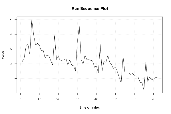
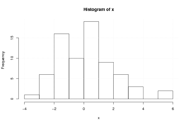
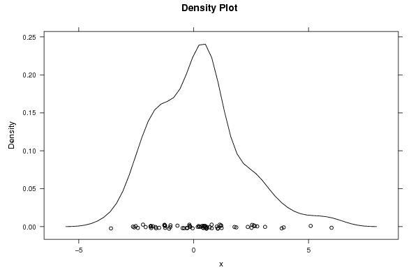
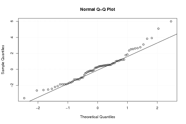
Dataseries X:

Download CSV

Histogram

Boxplots

0,306
0,788
2,354
2,656
1,216
6
3,918
2,542
2,766
2,516
1,776
1,854
0,78
1,186
1,048
0,43
-0,176
3,83
0,584
1,006
0,382
0,496
0,526
0,7
-0,18
0,558
-0,19
-0,284
-1,01
3,108
5,092
0,498
-0,046
1,19
0,554
0,56
0,466
0,396
-0,482
-0,296
-1,246
2,618
-1,022
0,422
0,176
1,134
0,218
-0,148
-0,708
-0,422
-1,074
-1,858
-2,644
1,048
-1,272
-1,252
-1,242
-1,506
-1,28
-1,638
-1,662
-1,868
-2,526
-2,584
-3,602
0,248
-2,43
-1,778
-2,206
-2,092
-1,88
-1,852

Summary of computational transaction
Raw Input	view raw input (R code)
Raw Output	view raw output of R engine
Computing time	6 seconds
R Server	'RServer@AstonUniversity' @ vre.aston.ac.uk

\begin{tabular}{lllllllll}
\hline
Summary of computational transaction \tabularnewline
Raw Input & view raw input (R code)  \tabularnewline
Raw Output & view raw output of R engine  \tabularnewline
Computing time & 6 seconds \tabularnewline
R Server & 'RServer@AstonUniversity' @ vre.aston.ac.uk \tabularnewline
\hline
\end{tabular}
%Source: https://freestatistics.org/blog/index.php?pk=53703&T=0

[TABLE]
[ROW][C]Summary of computational transaction[/C][/ROW]
[ROW][C]Raw Input[/C][C]view raw input (R code) [/C][/ROW]
[ROW][C]Raw Output[/C][C]view raw output of R engine [/C][/ROW]
[ROW][C]Computing time[/C][C]6 seconds[/C][/ROW]
[ROW][C]R Server[/C][C]'RServer@AstonUniversity' @ vre.aston.ac.uk[/C][/ROW]
[/TABLE]
Source: https://freestatistics.org/blog/index.php?pk=53703&T=0

Globally Unique Identifier (entire table): ba.freestatistics.org/blog/index.php?pk=53703&T=0

As an alternative you can also use a QR Code:

The GUIDs for individual cells are displayed in the table below:

Summary of computational transaction
Raw Input	view raw input (R code)
Raw Output	view raw output of R engine
Computing time	6 seconds
R Server	'RServer@AstonUniversity' @ vre.aston.ac.uk

Descriptive Statistics
# observations	72
minimum	-3.602
Q1	-1.2475
median	0.277
mean	0.187361111111111
Q3	1.048
maximum	6

\begin{tabular}{lllllllll}
\hline
Descriptive Statistics \tabularnewline
# observations & 72 \tabularnewline
minimum & -3.602 \tabularnewline
Q1 & -1.2475 \tabularnewline
median & 0.277 \tabularnewline
mean & 0.187361111111111 \tabularnewline
Q3 & 1.048 \tabularnewline
maximum & 6 \tabularnewline
\hline
\end{tabular}
%Source: https://freestatistics.org/blog/index.php?pk=53703&T=1

[TABLE]
[ROW][C]Descriptive Statistics[/C][/ROW]
[ROW][C]# observations[/C][C]72[/C][/ROW]
[ROW][C]minimum[/C][C]-3.602[/C][/ROW]
[ROW][C]Q1[/C][C]-1.2475[/C][/ROW]
[ROW][C]median[/C][C]0.277[/C][/ROW]
[ROW][C]mean[/C][C]0.187361111111111[/C][/ROW]
[ROW][C]Q3[/C][C]1.048[/C][/ROW]
[ROW][C]maximum[/C][C]6[/C][/ROW]
[/TABLE]
Source: https://freestatistics.org/blog/index.php?pk=53703&T=1

Globally Unique Identifier (entire table): ba.freestatistics.org/blog/index.php?pk=53703&T=1

As an alternative you can also use a QR Code:

The GUIDs for individual cells are displayed in the table below:

Descriptive Statistics
# observations	72
minimum	-3.602
Q1	-1.2475
median	0.277
mean	0.187361111111111
Q3	1.048
maximum	6

Figure 1

PNG link

Postscript link

PDF link

Figure 2

PNG link

Postscript link

PDF link

Figure 3

PNG link

Postscript link

PDF link

Figure 4

PNG link

Postscript link

PDF link

Figure 5

PNG link

Postscript link

PDF link

Figure 6

PNG link

Postscript link

PDF link

Figure 7

PNG link

Postscript link

PDF link

Parameters (Session):

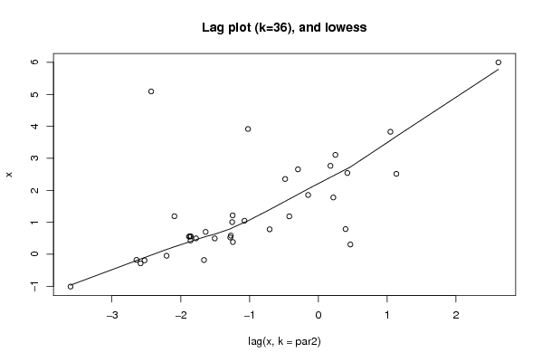
par1 = 0 ; par2 = 36 ;

Parameters (R input):

par1 = 0 ; par2 = 36 ;

R code (references can be found in the software module):

par1 <- as.numeric(par1)
par2 <- as.numeric(par2)
x <- as.ts(x)
library(lattice)
bitmap(file='pic1.png')
plot(x,type='l',main='Run Sequence Plot',xlab='time or index',ylab='value')
grid()
dev.off()
bitmap(file='pic2.png')
hist(x)
grid()
dev.off()
bitmap(file='pic3.png')
if (par1 > 0)
{
densityplot(~x,col='black',main=paste('Density Plot   bw = ',par1),bw=par1)
} else {
densityplot(~x,col='black',main='Density Plot')
}
dev.off()
bitmap(file='pic4.png')
qqnorm(x)
qqline(x)
grid()
dev.off()
if (par2 > 0)
{
bitmap(file='lagplot1.png')
dum <- cbind(lag(x,k=1),x)
dum
dum1 <- dum[2:length(x),]
dum1
z <- as.data.frame(dum1)
z
plot(z,main='Lag plot (k=1), lowess, and regression line')
lines(lowess(z))
abline(lm(z))
dev.off()
if (par2 > 1) {
bitmap(file='lagplotpar2.png')
dum <- cbind(lag(x,k=par2),x)
dum
dum1 <- dum[(par2+1):length(x),]
dum1
z <- as.data.frame(dum1)
z
mylagtitle <- 'Lag plot (k='
mylagtitle <- paste(mylagtitle,par2,sep='')
mylagtitle <- paste(mylagtitle,'), and lowess',sep='')
plot(z,main=mylagtitle)
lines(lowess(z))
dev.off()
}
bitmap(file='pic5.png')
acf(x,lag.max=par2,main='Autocorrelation Function')
grid()
dev.off()
}
summary(x)
load(file='createtable')
a<-table.start()
a<-table.row.start(a)
a<-table.element(a,'Descriptive Statistics',2,TRUE)
a<-table.row.end(a)
a<-table.row.start(a)
a<-table.element(a,'# observations',header=TRUE)
a<-table.element(a,length(x))
a<-table.row.end(a)
a<-table.row.start(a)
a<-table.element(a,'minimum',header=TRUE)
a<-table.element(a,min(x))
a<-table.row.end(a)
a<-table.row.start(a)
a<-table.element(a,'Q1',header=TRUE)
a<-table.element(a,quantile(x,0.25))
a<-table.row.end(a)
a<-table.row.start(a)
a<-table.element(a,'median',header=TRUE)
a<-table.element(a,median(x))
a<-table.row.end(a)
a<-table.row.start(a)
a<-table.element(a,'mean',header=TRUE)
a<-table.element(a,mean(x))
a<-table.row.end(a)
a<-table.row.start(a)
a<-table.element(a,'Q3',header=TRUE)
a<-table.element(a,quantile(x,0.75))
a<-table.row.end(a)
a<-table.row.start(a)
a<-table.element(a,'maximum',header=TRUE)
a<-table.element(a,max(x))
a<-table.row.end(a)
a<-table.end(a)
table.save(a,file='mytable.tab')

Free Statistics

Description of Statistical Computation

Tree of Dependent Computations

Dataset

Tables (Output of Computation)

Figures (Output of Computation)

Input Parameters & R Code