Free Statistics
of Irreproducible Research!
Description of Statistical Computation | |||||||||||||||||||||||||||||||||||||||||||||||||||||||||||||||||
|---|---|---|---|---|---|---|---|---|---|---|---|---|---|---|---|---|---|---|---|---|---|---|---|---|---|---|---|---|---|---|---|---|---|---|---|---|---|---|---|---|---|---|---|---|---|---|---|---|---|---|---|---|---|---|---|---|---|---|---|---|---|---|---|---|---|
| Author's title | |||||||||||||||||||||||||||||||||||||||||||||||||||||||||||||||||
| Author | *The author of this computation has been verified* | ||||||||||||||||||||||||||||||||||||||||||||||||||||||||||||||||
| R Software Module | rwasp_edabi.wasp | ||||||||||||||||||||||||||||||||||||||||||||||||||||||||||||||||
| Title produced by software | Bivariate Explorative Data Analysis | ||||||||||||||||||||||||||||||||||||||||||||||||||||||||||||||||
| Date of computation | Wed, 04 Nov 2009 10:45:28 -0700 | ||||||||||||||||||||||||||||||||||||||||||||||||||||||||||||||||
| Cite this page as follows | Statistical Computations at FreeStatistics.org, Office for Research Development and Education, URL https://freestatistics.org/blog/index.php?v=date/2009/Nov/04/t12573567847saojni8poiddi2.htm/, Retrieved Mon, 29 Apr 2024 12:31:46 +0000 | ||||||||||||||||||||||||||||||||||||||||||||||||||||||||||||||||
| Statistical Computations at FreeStatistics.org, Office for Research Development and Education, URL https://freestatistics.org/blog/index.php?pk=53760, Retrieved Mon, 29 Apr 2024 12:31:46 +0000 | |||||||||||||||||||||||||||||||||||||||||||||||||||||||||||||||||
| QR Codes: | |||||||||||||||||||||||||||||||||||||||||||||||||||||||||||||||||
|
| |||||||||||||||||||||||||||||||||||||||||||||||||||||||||||||||||
| Original text written by user: | |||||||||||||||||||||||||||||||||||||||||||||||||||||||||||||||||
| IsPrivate? | No (this computation is public) | ||||||||||||||||||||||||||||||||||||||||||||||||||||||||||||||||
| User-defined keywords | |||||||||||||||||||||||||||||||||||||||||||||||||||||||||||||||||
| Estimated Impact | 243 | ||||||||||||||||||||||||||||||||||||||||||||||||||||||||||||||||
Tree of Dependent Computations | |||||||||||||||||||||||||||||||||||||||||||||||||||||||||||||||||
| Family? (F = Feedback message, R = changed R code, M = changed R Module, P = changed Parameters, D = changed Data) | |||||||||||||||||||||||||||||||||||||||||||||||||||||||||||||||||
| F [Bivariate Explorative Data Analysis] [WS5] [2009-11-03 17:19:04] [eea7474c6df699240a34279975905c82] - D [Bivariate Explorative Data Analysis] [reeks X t.o.v Z] [2009-11-04 17:42:17] [cd6314e7e707a6546bd4604c9d1f2b69] - D [Bivariate Explorative Data Analysis] [reeks Y t.o.v. Z] [2009-11-04 17:45:28] [ea241b681aafed79da4b5b99fad98471] [Current] - D [Bivariate Explorative Data Analysis] [e(t) t.o.v. e'(t)] [2009-11-04 17:48:40] [cd6314e7e707a6546bd4604c9d1f2b69] - RMPD [Pearson Correlation] [correlatie e(t) e...] [2009-11-04 17:50:43] [cd6314e7e707a6546bd4604c9d1f2b69] - PD [Bivariate Explorative Data Analysis] [e(t) t.o.v. e'(t)] [2009-11-04 18:01:26] [cd6314e7e707a6546bd4604c9d1f2b69] | |||||||||||||||||||||||||||||||||||||||||||||||||||||||||||||||||
| Feedback Forum | |||||||||||||||||||||||||||||||||||||||||||||||||||||||||||||||||
Post a new message | |||||||||||||||||||||||||||||||||||||||||||||||||||||||||||||||||
Dataset | |||||||||||||||||||||||||||||||||||||||||||||||||||||||||||||||||
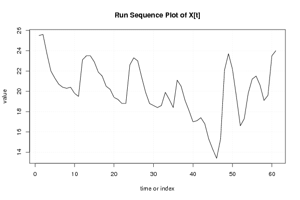
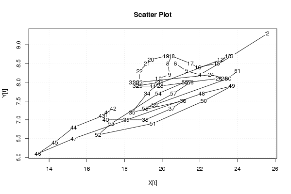
| Dataseries X: | |||||||||||||||||||||||||||||||||||||||||||||||||||||||||||||||||
25.5 25.6 23.7 22 21.3 20.7 20.4 20.3 20.4 19.8 19.5 23.1 23.5 23.5 22.9 21.9 21.5 20.5 20.2 19.4 19.2 18.8 18.8 22.6 23.3 23 21.4 19.9 18.8 18.6 18.4 18.6 19.9 19.2 18.4 21.1 20.5 19.1 18.1 17 17.1 17.4 16.8 15.3 14.3 13.4 15.3 22.1 23.7 22.2 19.5 16.6 17.3 19.8 21.2 21.5 20.6 19.1 19.6 23.5 24 | |||||||||||||||||||||||||||||||||||||||||||||||||||||||||||||||||
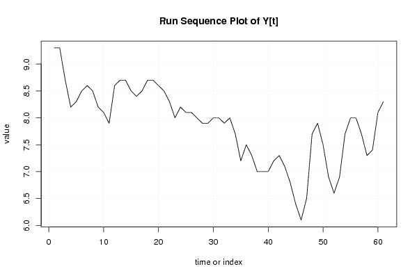
| Dataseries Y: | |||||||||||||||||||||||||||||||||||||||||||||||||||||||||||||||||
9,3 9,3 8,7 8,2 8,3 8,5 8,6 8,5 8,2 8,1 7,9 8,6 8,7 8,7 8,5 8,4 8,5 8,7 8,7 8,6 8,5 8,3 8 8,2 8,1 8,1 8 7,9 7,9 8 8 7,9 8 7,7 7,2 7,5 7,3 7 7 7 7,2 7,3 7,1 6,8 6,4 6,1 6,5 7,7 7,9 7,5 6,9 6,6 6,9 7,7 8 8 7,7 7,3 7,4 8,1 8,3 | |||||||||||||||||||||||||||||||||||||||||||||||||||||||||||||||||
Tables (Output of Computation) | |||||||||||||||||||||||||||||||||||||||||||||||||||||||||||||||||
| |||||||||||||||||||||||||||||||||||||||||||||||||||||||||||||||||
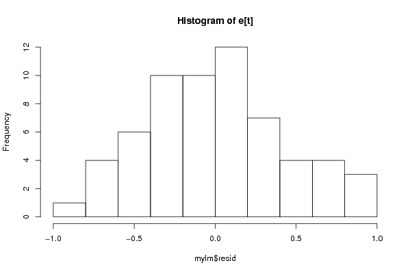
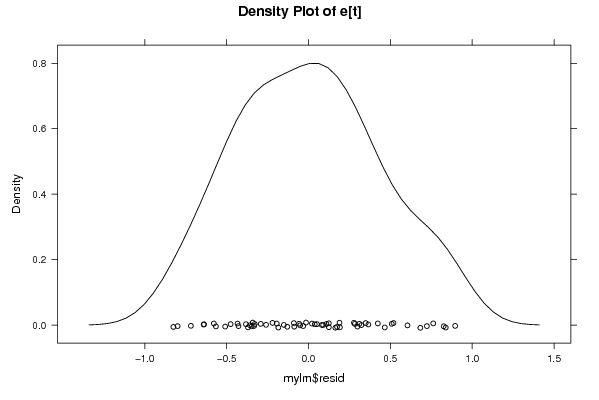
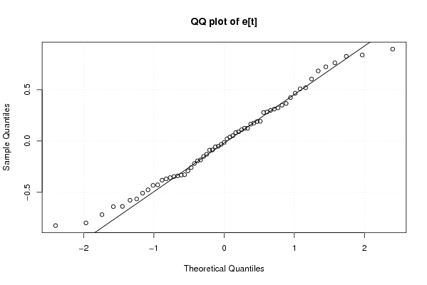
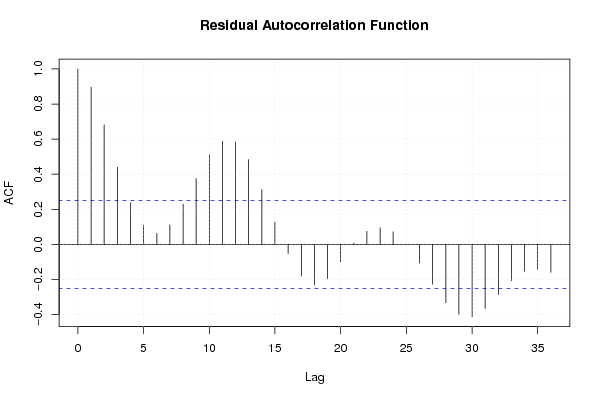
Figures (Output of Computation) | |||||||||||||||||||||||||||||||||||||||||||||||||||||||||||||||||
Input Parameters & R Code | |||||||||||||||||||||||||||||||||||||||||||||||||||||||||||||||||
| Parameters (Session): | |||||||||||||||||||||||||||||||||||||||||||||||||||||||||||||||||
| par1 = 0 ; par2 = 36 ; | |||||||||||||||||||||||||||||||||||||||||||||||||||||||||||||||||
| Parameters (R input): | |||||||||||||||||||||||||||||||||||||||||||||||||||||||||||||||||
| par1 = 0 ; par2 = 36 ; | |||||||||||||||||||||||||||||||||||||||||||||||||||||||||||||||||
| R code (references can be found in the software module): | |||||||||||||||||||||||||||||||||||||||||||||||||||||||||||||||||
par1 <- as.numeric(par1) | |||||||||||||||||||||||||||||||||||||||||||||||||||||||||||||||||