Free Statistics
of Irreproducible Research!
Description of Statistical Computation | |||||||||||||||||||||||||||||||||||||||||||||||||||||||||||||||||
|---|---|---|---|---|---|---|---|---|---|---|---|---|---|---|---|---|---|---|---|---|---|---|---|---|---|---|---|---|---|---|---|---|---|---|---|---|---|---|---|---|---|---|---|---|---|---|---|---|---|---|---|---|---|---|---|---|---|---|---|---|---|---|---|---|---|
| Author's title | |||||||||||||||||||||||||||||||||||||||||||||||||||||||||||||||||
| Author | *The author of this computation has been verified* | ||||||||||||||||||||||||||||||||||||||||||||||||||||||||||||||||
| R Software Module | rwasp_edabi.wasp | ||||||||||||||||||||||||||||||||||||||||||||||||||||||||||||||||
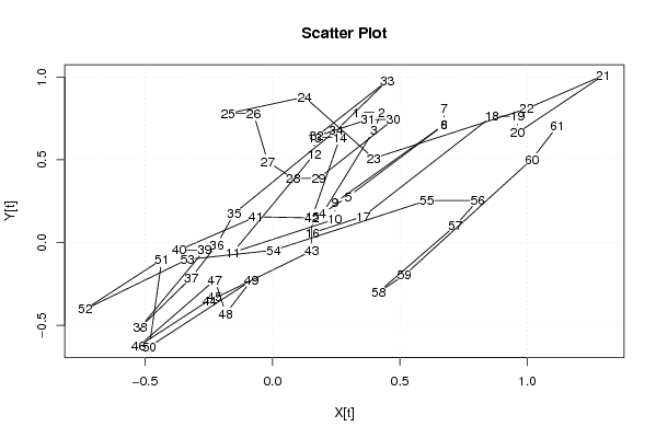
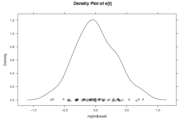
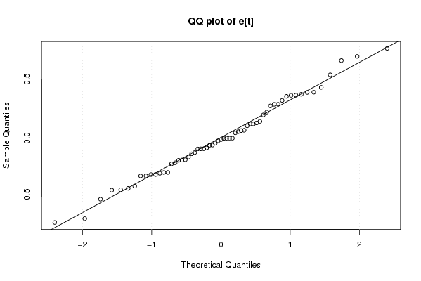
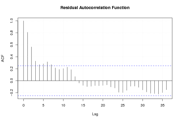
| Title produced by software | Bivariate Explorative Data Analysis | ||||||||||||||||||||||||||||||||||||||||||||||||||||||||||||||||
| Date of computation | Wed, 04 Nov 2009 10:48:40 -0700 | ||||||||||||||||||||||||||||||||||||||||||||||||||||||||||||||||
| Cite this page as follows | Statistical Computations at FreeStatistics.org, Office for Research Development and Education, URL https://freestatistics.org/blog/index.php?v=date/2009/Nov/04/t1257356979ew3ykm9005terby.htm/, Retrieved Mon, 29 Apr 2024 09:43:24 +0000 | ||||||||||||||||||||||||||||||||||||||||||||||||||||||||||||||||
| Statistical Computations at FreeStatistics.org, Office for Research Development and Education, URL https://freestatistics.org/blog/index.php?pk=53762, Retrieved Mon, 29 Apr 2024 09:43:24 +0000 | |||||||||||||||||||||||||||||||||||||||||||||||||||||||||||||||||
| QR Codes: | |||||||||||||||||||||||||||||||||||||||||||||||||||||||||||||||||
|
| |||||||||||||||||||||||||||||||||||||||||||||||||||||||||||||||||
| Original text written by user: | |||||||||||||||||||||||||||||||||||||||||||||||||||||||||||||||||
| IsPrivate? | No (this computation is public) | ||||||||||||||||||||||||||||||||||||||||||||||||||||||||||||||||
| User-defined keywords | |||||||||||||||||||||||||||||||||||||||||||||||||||||||||||||||||
| Estimated Impact | 144 | ||||||||||||||||||||||||||||||||||||||||||||||||||||||||||||||||
Tree of Dependent Computations | |||||||||||||||||||||||||||||||||||||||||||||||||||||||||||||||||
| Family? (F = Feedback message, R = changed R code, M = changed R Module, P = changed Parameters, D = changed Data) | |||||||||||||||||||||||||||||||||||||||||||||||||||||||||||||||||
| F [Bivariate Explorative Data Analysis] [WS5] [2009-11-03 17:19:04] [eea7474c6df699240a34279975905c82] - D [Bivariate Explorative Data Analysis] [reeks X t.o.v Z] [2009-11-04 17:42:17] [cd6314e7e707a6546bd4604c9d1f2b69] - D [Bivariate Explorative Data Analysis] [reeks Y t.o.v. Z] [2009-11-04 17:45:28] [cd6314e7e707a6546bd4604c9d1f2b69] - D [Bivariate Explorative Data Analysis] [e(t) t.o.v. e'(t)] [2009-11-04 17:48:40] [ea241b681aafed79da4b5b99fad98471] [Current] - RMPD [Pearson Correlation] [correlatie e(t) e...] [2009-11-04 17:50:43] [cd6314e7e707a6546bd4604c9d1f2b69] - PD [Bivariate Explorative Data Analysis] [e(t) t.o.v. e'(t)] [2009-11-04 18:01:26] [cd6314e7e707a6546bd4604c9d1f2b69] | |||||||||||||||||||||||||||||||||||||||||||||||||||||||||||||||||
| Feedback Forum | |||||||||||||||||||||||||||||||||||||||||||||||||||||||||||||||||
Post a new message | |||||||||||||||||||||||||||||||||||||||||||||||||||||||||||||||||
Dataset | |||||||||||||||||||||||||||||||||||||||||||||||||||||||||||||||||
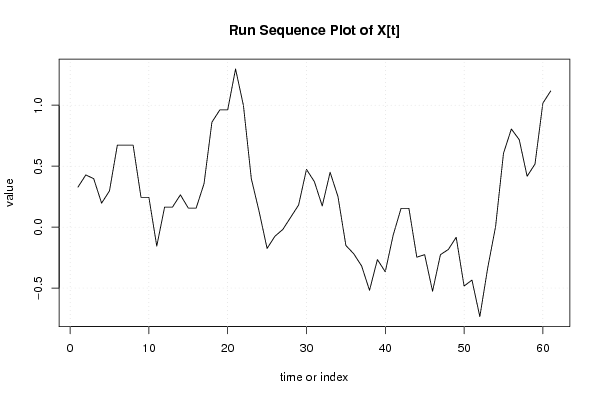
| Dataseries X: | |||||||||||||||||||||||||||||||||||||||||||||||||||||||||||||||||
0,328553678 0,428553678 0,397030204 0,197030204 0,297030204 0,673258107 0,673258107 0,673258107 0,245092359 0,245092359 -0,154907641 0,164988767 0,164988767 0,264988767 0,156719426 0,156719426 0,356719426 0,861113078 0,961113078 0,961113078 1,297548166 0,997548166 0,397548166 0,125713914 -0,174286086 -0,074286086 -0,018472552 0,081527448 0,181527448 0,47377607 0,37377607 0,17377607 0,450003973 0,250003973 -0,149996027 -0,218472552 -0,318472552 -0,518472552 -0,266016745 -0,366016745 -0,066016745 0,153879662 0,153879662 -0,246120338 -0,225705968 -0,525705968 -0,225705968 -0,183073389 -0,083073389 -0,483073389 -0,433975308 -0,733975308 -0,333975308 0,005299544 0,605299544 0,805299544 0,717444574 0,417444574 0,517444574 1,017444574 1,117444574 | |||||||||||||||||||||||||||||||||||||||||||||||||||||||||||||||||
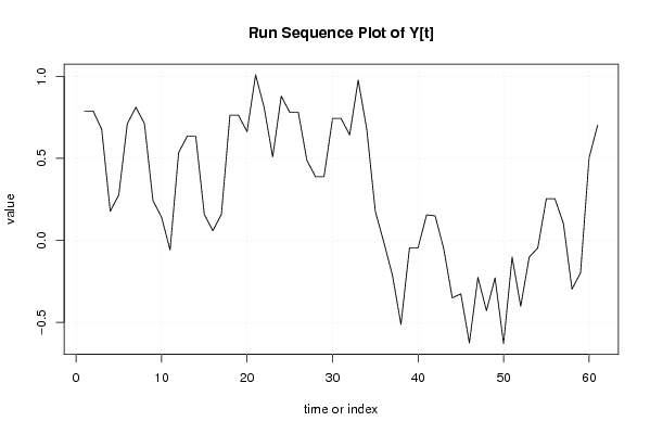
| Dataseries Y: | |||||||||||||||||||||||||||||||||||||||||||||||||||||||||||||||||
0,788105644 0,788105644 0,677096311 0,177096311 0,277096311 0,710961413 0,810961413 0,710961413 0,240877703 0,140877703 -0,059122297 0,534575384 0,634575384 0,634575384 0,158189355 0,058189355 0,158189355 0,762138167 0,762138167 0,662138167 1,008607906 0,808607906 0,508607906 0,878691617 0,778691617 0,778691617 0,487347443 0,387347443 0,387347443 0,742473008 0,742473008 0,642473008 0,97633811 0,67633811 0,17633811 -0,012652557 -0,212652557 -0,512652557 -0,044922354 -0,044922354 0,155077646 0,148775327 -0,051224673 -0,351224673 -0,326015397 -0,626015397 -0,226015397 -0,429206007 -0,229206007 -0,629206007 -0,102401426 -0,402401426 -0,102401426 -0,046517659 0,253482341 0,253482341 0,102305587 -0,297694413 -0,197694413 0,502305587 0,702305587 | |||||||||||||||||||||||||||||||||||||||||||||||||||||||||||||||||
Tables (Output of Computation) | |||||||||||||||||||||||||||||||||||||||||||||||||||||||||||||||||
| |||||||||||||||||||||||||||||||||||||||||||||||||||||||||||||||||
Figures (Output of Computation) | |||||||||||||||||||||||||||||||||||||||||||||||||||||||||||||||||
Input Parameters & R Code | |||||||||||||||||||||||||||||||||||||||||||||||||||||||||||||||||
| Parameters (Session): | |||||||||||||||||||||||||||||||||||||||||||||||||||||||||||||||||
| par1 = 0 ; par2 = 36 ; | |||||||||||||||||||||||||||||||||||||||||||||||||||||||||||||||||
| Parameters (R input): | |||||||||||||||||||||||||||||||||||||||||||||||||||||||||||||||||
| par1 = 0 ; par2 = 36 ; | |||||||||||||||||||||||||||||||||||||||||||||||||||||||||||||||||
| R code (references can be found in the software module): | |||||||||||||||||||||||||||||||||||||||||||||||||||||||||||||||||
par1 <- as.numeric(par1) | |||||||||||||||||||||||||||||||||||||||||||||||||||||||||||||||||