Free Statistics
of Irreproducible Research!
Description of Statistical Computation | |||||||||||||||||||||||||||||||||||||||||||||||||||||||||||||||||
|---|---|---|---|---|---|---|---|---|---|---|---|---|---|---|---|---|---|---|---|---|---|---|---|---|---|---|---|---|---|---|---|---|---|---|---|---|---|---|---|---|---|---|---|---|---|---|---|---|---|---|---|---|---|---|---|---|---|---|---|---|---|---|---|---|---|
| Author's title | |||||||||||||||||||||||||||||||||||||||||||||||||||||||||||||||||
| Author | *The author of this computation has been verified* | ||||||||||||||||||||||||||||||||||||||||||||||||||||||||||||||||
| R Software Module | rwasp_edabi.wasp | ||||||||||||||||||||||||||||||||||||||||||||||||||||||||||||||||
| Title produced by software | Bivariate Explorative Data Analysis | ||||||||||||||||||||||||||||||||||||||||||||||||||||||||||||||||
| Date of computation | Wed, 04 Nov 2009 10:53:08 -0700 | ||||||||||||||||||||||||||||||||||||||||||||||||||||||||||||||||
| Cite this page as follows | Statistical Computations at FreeStatistics.org, Office for Research Development and Education, URL https://freestatistics.org/blog/index.php?v=date/2009/Nov/04/t12573572640l6medru0vx1c2i.htm/, Retrieved Mon, 29 Apr 2024 15:24:35 +0000 | ||||||||||||||||||||||||||||||||||||||||||||||||||||||||||||||||
| Statistical Computations at FreeStatistics.org, Office for Research Development and Education, URL https://freestatistics.org/blog/index.php?pk=53765, Retrieved Mon, 29 Apr 2024 15:24:35 +0000 | |||||||||||||||||||||||||||||||||||||||||||||||||||||||||||||||||
| QR Codes: | |||||||||||||||||||||||||||||||||||||||||||||||||||||||||||||||||
|
| |||||||||||||||||||||||||||||||||||||||||||||||||||||||||||||||||
| Original text written by user: | |||||||||||||||||||||||||||||||||||||||||||||||||||||||||||||||||
| IsPrivate? | No (this computation is public) | ||||||||||||||||||||||||||||||||||||||||||||||||||||||||||||||||
| User-defined keywords | |||||||||||||||||||||||||||||||||||||||||||||||||||||||||||||||||
| Estimated Impact | 113 | ||||||||||||||||||||||||||||||||||||||||||||||||||||||||||||||||
Tree of Dependent Computations | |||||||||||||||||||||||||||||||||||||||||||||||||||||||||||||||||
| Family? (F = Feedback message, R = changed R code, M = changed R Module, P = changed Parameters, D = changed Data) | |||||||||||||||||||||||||||||||||||||||||||||||||||||||||||||||||
| - [Bivariate Explorative Data Analysis] [WS5.5] [2009-11-04 17:53:08] [dd4f17965cad1d38de7a1c062d32d75d] [Current] | |||||||||||||||||||||||||||||||||||||||||||||||||||||||||||||||||
| Feedback Forum | |||||||||||||||||||||||||||||||||||||||||||||||||||||||||||||||||
Post a new message | |||||||||||||||||||||||||||||||||||||||||||||||||||||||||||||||||
Dataset | |||||||||||||||||||||||||||||||||||||||||||||||||||||||||||||||||
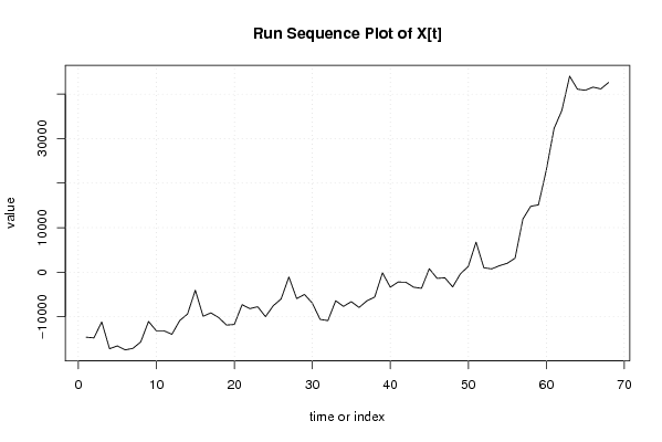
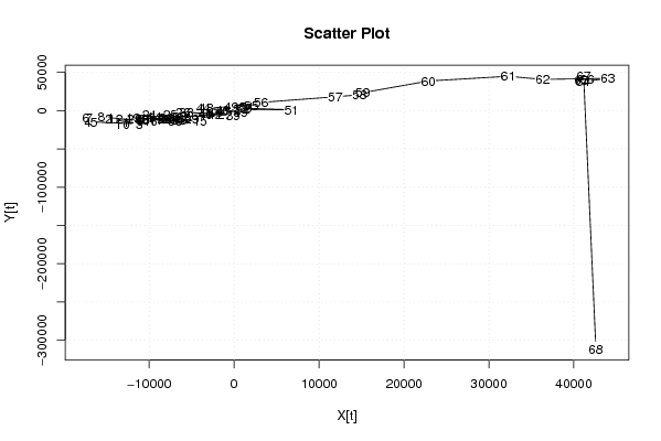
| Dataseries X: | |||||||||||||||||||||||||||||||||||||||||||||||||||||||||||||||||
-14592,498 -14749,83 -11156,16 -17184,822 -16545,82 -17444,154 -17099,494 -15654,83 -11063,164 -13154,828 -13161,16 -13948,494 -10852,162 -9392,162 -4035,162 -9891,16 -9131,16 -10197,824 -11863,16 -11729,16 -7285,494 -8177,828 -7750,828 -9981,496 -7517,164 -6005,498 -1075,498 -5927,498 -4997,496 -6932,492 -10592,156 -10866,154 -6412,488 -7672,156 -6610,49 -7920,824 -6428,158 -5585,824 -133,156 -3363,49 -2202,822 -2256,486 -3363,488 -3620,154 783,514 -1380,152 -1259,818 -3304,82 -347,822 1289,178 6757,514 1001,516 745,518 1461,516 2010,842 3153,508 11929,844 14782,516 15136,518 22871,182 32275,176 36322,172 44015,504 41091,172 40859,174 41557,84 41163,17 42609,836 | |||||||||||||||||||||||||||||||||||||||||||||||||||||||||||||||||
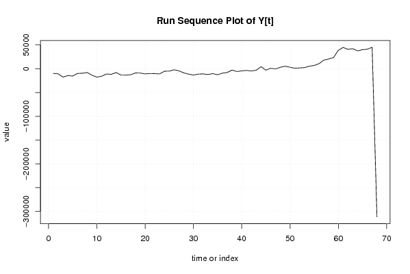
| Dataseries Y: | |||||||||||||||||||||||||||||||||||||||||||||||||||||||||||||||||
-9879,41 -10788,3 -17642,546 -14437,08 -15375,902 -10005,122 -9551,41 -7988,232 -13723,944 -17598,3 -15783,122 -11085,766 -11790,766 -8022,766 -13348,3 -13524,3 -12618,012 -8935,3 -9100,3 -10968,122 -10056,944 -10411,944 -10946,588 -5283,232 -5128,054 -2249,054 -4387,054 -8762,588 -11380,656 -13290,368 -11371,902 -10899,724 -12171,368 -10352,19 -12691,012 -9346,834 -7929,012 -2859,368 -5897,19 -4573,546 -3579,258 -4843,724 -3116,902 4224,742 -2958,436 940,386 -455,08 3108,454 5254,454 3068,742 1027,208 1686,674 2374,208 5331,166 6855,344 10646,632 18059,208 20561,674 23339,386 38642,988 44831,056 40739,412 42120,056 37655,522 40053,7 41048,59 45168,768 -311562,65 | |||||||||||||||||||||||||||||||||||||||||||||||||||||||||||||||||
Tables (Output of Computation) | |||||||||||||||||||||||||||||||||||||||||||||||||||||||||||||||||
| |||||||||||||||||||||||||||||||||||||||||||||||||||||||||||||||||
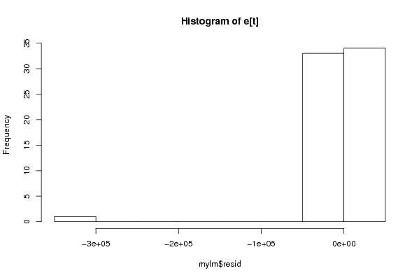
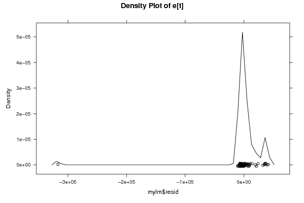
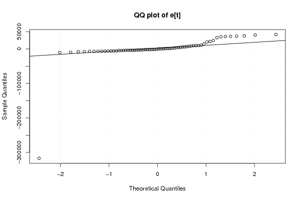
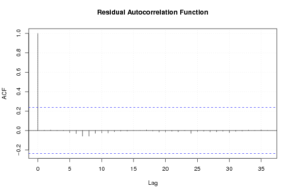
Figures (Output of Computation) | |||||||||||||||||||||||||||||||||||||||||||||||||||||||||||||||||
Input Parameters & R Code | |||||||||||||||||||||||||||||||||||||||||||||||||||||||||||||||||
| Parameters (Session): | |||||||||||||||||||||||||||||||||||||||||||||||||||||||||||||||||
| par1 = 0 ; par2 = 36 ; | |||||||||||||||||||||||||||||||||||||||||||||||||||||||||||||||||
| Parameters (R input): | |||||||||||||||||||||||||||||||||||||||||||||||||||||||||||||||||
| par1 = 0 ; par2 = 36 ; | |||||||||||||||||||||||||||||||||||||||||||||||||||||||||||||||||
| R code (references can be found in the software module): | |||||||||||||||||||||||||||||||||||||||||||||||||||||||||||||||||
par1 <- as.numeric(par1) | |||||||||||||||||||||||||||||||||||||||||||||||||||||||||||||||||