Free Statistics
of Irreproducible Research!
Description of Statistical Computation | |||||||||||||||||||||
|---|---|---|---|---|---|---|---|---|---|---|---|---|---|---|---|---|---|---|---|---|---|
| Author's title | |||||||||||||||||||||
| Author | *The author of this computation has been verified* | ||||||||||||||||||||
| R Software Module | rwasp_cloud.wasp | ||||||||||||||||||||
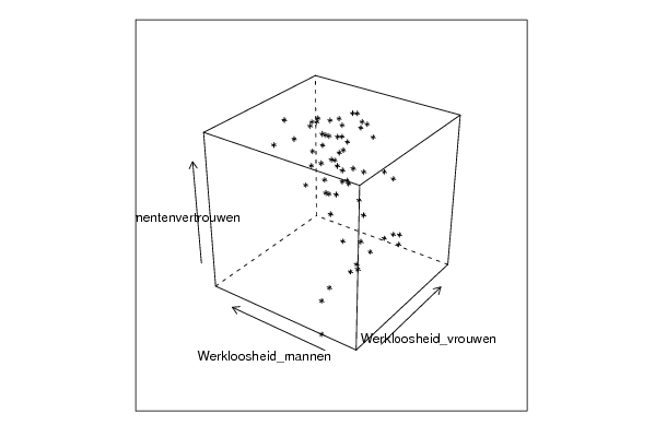
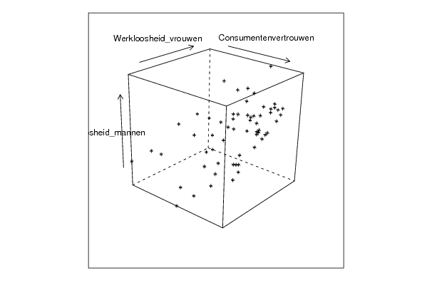
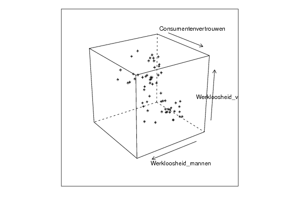
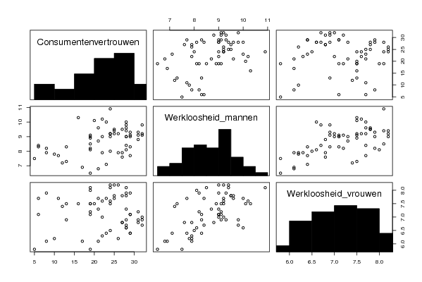
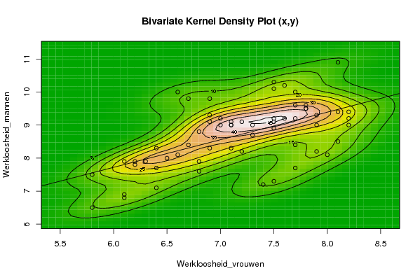
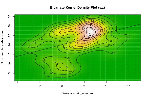
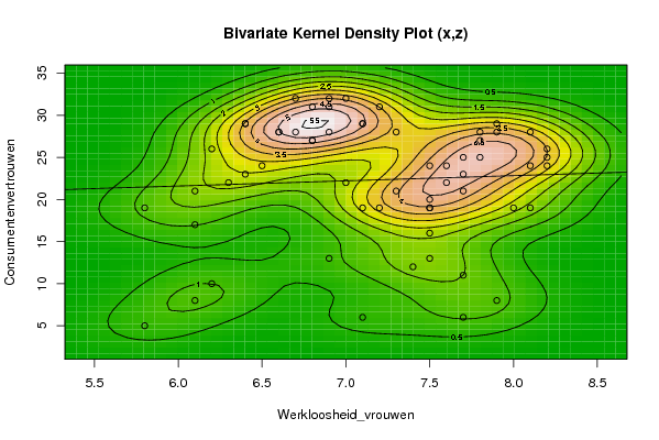
| Title produced by software | Trivariate Scatterplots | ||||||||||||||||||||
| Date of computation | Wed, 04 Nov 2009 11:44:04 -0700 | ||||||||||||||||||||
| Cite this page as follows | Statistical Computations at FreeStatistics.org, Office for Research Development and Education, URL https://freestatistics.org/blog/index.php?v=date/2009/Nov/04/t1257360293ag673em48hvvrac.htm/, Retrieved Mon, 29 Apr 2024 08:25:17 +0000 | ||||||||||||||||||||
| Statistical Computations at FreeStatistics.org, Office for Research Development and Education, URL https://freestatistics.org/blog/index.php?pk=53793, Retrieved Mon, 29 Apr 2024 08:25:17 +0000 | |||||||||||||||||||||
| QR Codes: | |||||||||||||||||||||
|
| |||||||||||||||||||||
| Original text written by user: | |||||||||||||||||||||
| IsPrivate? | No (this computation is public) | ||||||||||||||||||||
| User-defined keywords | |||||||||||||||||||||
| Estimated Impact | 149 | ||||||||||||||||||||
Tree of Dependent Computations | |||||||||||||||||||||
| Family? (F = Feedback message, R = changed R code, M = changed R Module, P = changed Parameters, D = changed Data) | |||||||||||||||||||||
| - [Trivariate Scatterplots] [SHW_WS5] [2009-10-29 16:26:54] [8b1aef4e7013bd33fbc2a5833375c5f5] - MPD [Trivariate Scatterplots] [WS5(5)] [2009-11-04 18:44:04] [5edea6bc5a9a9483633d9320282a2734] [Current] | |||||||||||||||||||||
| Feedback Forum | |||||||||||||||||||||
Post a new message | |||||||||||||||||||||
Dataset | |||||||||||||||||||||
| Dataseries X: | |||||||||||||||||||||
8,1 7,7 7,5 7,6 7,8 7,8 7,8 7,5 7,5 7,1 7,5 7,5 7,6 7,7 7,7 7,9 8,1 8,2 8,2 8,2 7,9 7,3 6,9 6,6 6,7 6,9 7 7,1 7,2 7,1 6,9 7 6,8 6,4 6,7 6,6 6,4 6,3 6,2 6,5 6,8 6,8 6,4 6,1 5,8 6,1 7,2 7,3 6,9 6,1 5,8 6,2 7,1 7,7 7,9 7,7 7,4 7,5 8 8,1 | |||||||||||||||||||||
| Dataseries Y: | |||||||||||||||||||||
10,9 10 9,2 9,2 9,5 9,6 9,5 9,1 8,9 9 10,1 10,3 10,2 9,6 9,2 9,3 9,4 9,4 9,2 9 9 9 9,8 10 9,8 9,3 9 9 9,1 9,1 9,1 9,2 8,8 8,3 8,4 8,1 7,7 7,9 7,9 8 7,9 7,6 7,1 6,8 6,5 6,9 8,2 8,7 8,3 7,9 7,5 7,8 8,3 8,4 8,2 7,7 7,2 7,3 8,1 8,5 | |||||||||||||||||||||
| Dataseries Z: | |||||||||||||||||||||
24 23 24 24 27 28 25 19 19 19 20 16 22 21 25 29 28 25 26 24 28 28 28 28 32 31 22 29 31 29 32 32 31 29 28 28 29 22 26 24 27 27 23 21 19 17 19 21 13 8 5 10 6 6 8 11 12 13 19 19 | |||||||||||||||||||||
Tables (Output of Computation) | |||||||||||||||||||||
| |||||||||||||||||||||
Figures (Output of Computation) | |||||||||||||||||||||
Input Parameters & R Code | |||||||||||||||||||||
| Parameters (Session): | |||||||||||||||||||||
| par1 = 50 ; par2 = 50 ; par3 = Y ; par4 = Y ; par5 = Werkloosheid_vrouwen ; par6 = Werkloosheid_mannen ; par7 = Consumentenvertrouwen ; | |||||||||||||||||||||
| Parameters (R input): | |||||||||||||||||||||
| par1 = 50 ; par2 = 50 ; par3 = Y ; par4 = Y ; par5 = Werkloosheid_vrouwen ; par6 = Werkloosheid_mannen ; par7 = Consumentenvertrouwen ; | |||||||||||||||||||||
| R code (references can be found in the software module): | |||||||||||||||||||||
x <- array(x,dim=c(length(x),1)) | |||||||||||||||||||||