Free Statistics
of Irreproducible Research!
Description of Statistical Computation | |||||||||||||||||||||||||||||||||||||||||||||||||||||||||||||||||
|---|---|---|---|---|---|---|---|---|---|---|---|---|---|---|---|---|---|---|---|---|---|---|---|---|---|---|---|---|---|---|---|---|---|---|---|---|---|---|---|---|---|---|---|---|---|---|---|---|---|---|---|---|---|---|---|---|---|---|---|---|---|---|---|---|---|
| Author's title | |||||||||||||||||||||||||||||||||||||||||||||||||||||||||||||||||
| Author | *The author of this computation has been verified* | ||||||||||||||||||||||||||||||||||||||||||||||||||||||||||||||||
| R Software Module | rwasp_edabi.wasp | ||||||||||||||||||||||||||||||||||||||||||||||||||||||||||||||||
| Title produced by software | Bivariate Explorative Data Analysis | ||||||||||||||||||||||||||||||||||||||||||||||||||||||||||||||||
| Date of computation | Wed, 04 Nov 2009 12:12:21 -0700 | ||||||||||||||||||||||||||||||||||||||||||||||||||||||||||||||||
| Cite this page as follows | Statistical Computations at FreeStatistics.org, Office for Research Development and Education, URL https://freestatistics.org/blog/index.php?v=date/2009/Nov/04/t1257362042tyzg6jd2o1o2mhd.htm/, Retrieved Mon, 29 Apr 2024 09:10:01 +0000 | ||||||||||||||||||||||||||||||||||||||||||||||||||||||||||||||||
| Statistical Computations at FreeStatistics.org, Office for Research Development and Education, URL https://freestatistics.org/blog/index.php?pk=53808, Retrieved Mon, 29 Apr 2024 09:10:01 +0000 | |||||||||||||||||||||||||||||||||||||||||||||||||||||||||||||||||
| QR Codes: | |||||||||||||||||||||||||||||||||||||||||||||||||||||||||||||||||
|
| |||||||||||||||||||||||||||||||||||||||||||||||||||||||||||||||||
| Original text written by user: | |||||||||||||||||||||||||||||||||||||||||||||||||||||||||||||||||
| IsPrivate? | No (this computation is public) | ||||||||||||||||||||||||||||||||||||||||||||||||||||||||||||||||
| User-defined keywords | ws5benrmldg | ||||||||||||||||||||||||||||||||||||||||||||||||||||||||||||||||
| Estimated Impact | 126 | ||||||||||||||||||||||||||||||||||||||||||||||||||||||||||||||||
Tree of Dependent Computations | |||||||||||||||||||||||||||||||||||||||||||||||||||||||||||||||||
| Family? (F = Feedback message, R = changed R code, M = changed R Module, P = changed Parameters, D = changed Data) | |||||||||||||||||||||||||||||||||||||||||||||||||||||||||||||||||
| - [Partial Correlation] [WS 5: partial cor...] [2009-11-03 20:50:00] [7c2a5b25a196bd646844b8f5223c9b3e] - RMPD [Bivariate Explorative Data Analysis] [WS 5: Bivariate E...] [2009-11-04 18:47:17] [7c2a5b25a196bd646844b8f5223c9b3e] - D [Bivariate Explorative Data Analysis] [WS 5: Bivariate E...] [2009-11-04 19:12:21] [3d2053c5f7c50d3c075d87ce0bd87294] [Current] | |||||||||||||||||||||||||||||||||||||||||||||||||||||||||||||||||
| Feedback Forum | |||||||||||||||||||||||||||||||||||||||||||||||||||||||||||||||||
Post a new message | |||||||||||||||||||||||||||||||||||||||||||||||||||||||||||||||||
Dataset | |||||||||||||||||||||||||||||||||||||||||||||||||||||||||||||||||
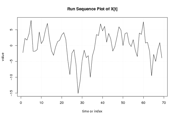
| Dataseries X: | |||||||||||||||||||||||||||||||||||||||||||||||||||||||||||||||||
-2,225348423 2,257563984 1,740476391 3,706301205 7,959396904 -1,810786388 -1,764228405 -1,270419804 4,26994678 0,614671842 1,706301205 4,797930568 6,99357209 2,027747276 -1,627527662 -3,076264883 -0,444268937 1,268460179 1,670639417 3,325914355 4,085201453 1,936117913 -4,638423857 -9,15551145 -2,385328158 -1,30459499 -5,936590936 -15,08567448 -11,20058283 -4,660216246 -1,464574724 -3,7751246 -3,20058283 -10,00494131 -3,315491184 -1,004941308 3,454692108 3,201596409 6,833592356 4,627054639 6,052512869 1,07579186 3,822696161 2,086688055 -1,740949414 -0,362049167 2,580496656 5,901942727 4,867767541 -0,017324105 3,810313364 4,051026267 0,672126019 -0,293698795 1,855384745 -1,43188614 -3,444268937 3,945527506 3,541861665 7,506199877 0,816749754 1,000008479 -1,770174813 -9,549075061 -2,783250246 -4,981417326 -1,341050742 0,916057116 -3,913759591 | |||||||||||||||||||||||||||||||||||||||||||||||||||||||||||||||||
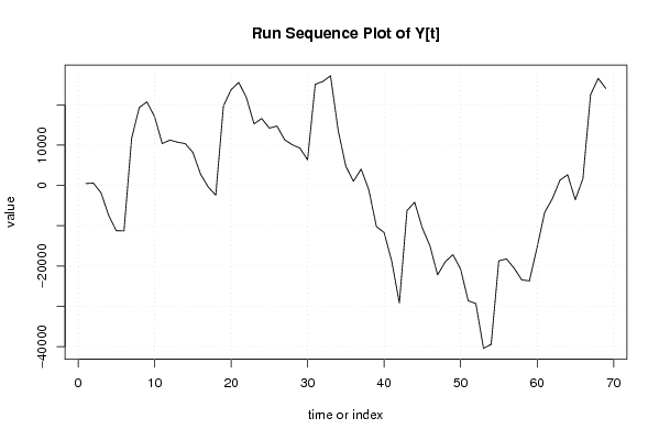
| Dataseries Y: | |||||||||||||||||||||||||||||||||||||||||||||||||||||||||||||||||
453,76 567,15 -1861,46 -7454,68 -11242,01 -11289,29 11715,62 19336,27 20729,84 17062,92 10369,32 11258,72 10721,21 10375,43 8202,51 2834,34 -371,69 -2429,58 19711,67 23745,59 25554,61 21797,03 15266,24 16605,63 14210,92 14714,05 11338,08 10074,50 9246,14 6347,71 25088,21 25798,35 27194,14 13649,64 4755,79 1004,64 4035,07 -1054,60 -10228,63 -11699,39 -18817,18 -29199,23 -6246,90 -4201,96 -10585,42 -15033,13 -22236,31 -18963,19 -17206,41 -20744,05 -28649,59 -29339,61 -40442,91 -39478,68 -18740,10 -18252,00 -20542,69 -23465,13 -23725,81 -15453,46 -6685,61 -3334,80 1292,91 2637,62 -3574,61 1701,23 22560,80 26551,57 24040,85 | |||||||||||||||||||||||||||||||||||||||||||||||||||||||||||||||||
Tables (Output of Computation) | |||||||||||||||||||||||||||||||||||||||||||||||||||||||||||||||||
| |||||||||||||||||||||||||||||||||||||||||||||||||||||||||||||||||
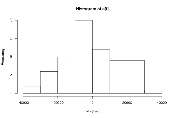
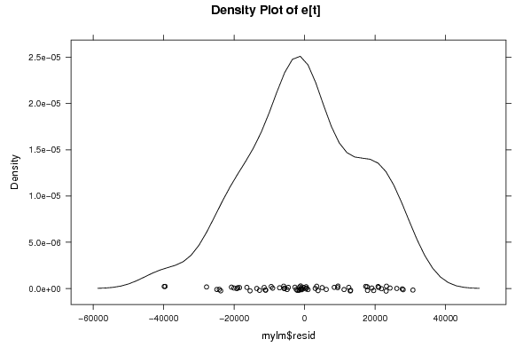
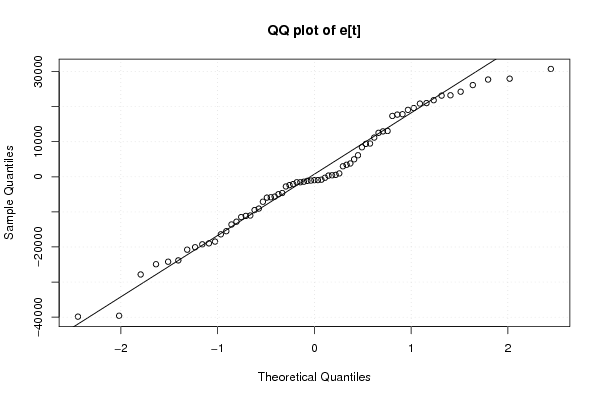
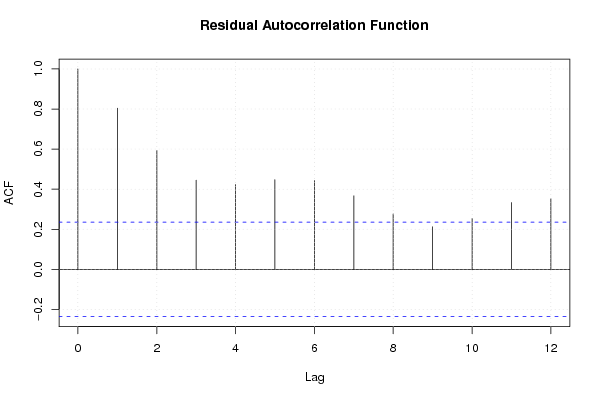
Figures (Output of Computation) | |||||||||||||||||||||||||||||||||||||||||||||||||||||||||||||||||
Input Parameters & R Code | |||||||||||||||||||||||||||||||||||||||||||||||||||||||||||||||||
| Parameters (Session): | |||||||||||||||||||||||||||||||||||||||||||||||||||||||||||||||||
| par1 = 0 ; par2 = 12 ; | |||||||||||||||||||||||||||||||||||||||||||||||||||||||||||||||||
| Parameters (R input): | |||||||||||||||||||||||||||||||||||||||||||||||||||||||||||||||||
| par1 = 0 ; par2 = 12 ; | |||||||||||||||||||||||||||||||||||||||||||||||||||||||||||||||||
| R code (references can be found in the software module): | |||||||||||||||||||||||||||||||||||||||||||||||||||||||||||||||||
par1 <- as.numeric(par1) | |||||||||||||||||||||||||||||||||||||||||||||||||||||||||||||||||