Free Statistics
of Irreproducible Research!
Description of Statistical Computation | |||||||||||||||||||||||||||||||||||||||||||||||||||||||||||||||||
|---|---|---|---|---|---|---|---|---|---|---|---|---|---|---|---|---|---|---|---|---|---|---|---|---|---|---|---|---|---|---|---|---|---|---|---|---|---|---|---|---|---|---|---|---|---|---|---|---|---|---|---|---|---|---|---|---|---|---|---|---|---|---|---|---|---|
| Author's title | |||||||||||||||||||||||||||||||||||||||||||||||||||||||||||||||||
| Author | *The author of this computation has been verified* | ||||||||||||||||||||||||||||||||||||||||||||||||||||||||||||||||
| R Software Module | rwasp_edabi.wasp | ||||||||||||||||||||||||||||||||||||||||||||||||||||||||||||||||
| Title produced by software | Bivariate Explorative Data Analysis | ||||||||||||||||||||||||||||||||||||||||||||||||||||||||||||||||
| Date of computation | Wed, 04 Nov 2009 14:47:53 -0700 | ||||||||||||||||||||||||||||||||||||||||||||||||||||||||||||||||
| Cite this page as follows | Statistical Computations at FreeStatistics.org, Office for Research Development and Education, URL https://freestatistics.org/blog/index.php?v=date/2009/Nov/04/t1257371584ov65insz6nipmsv.htm/, Retrieved Mon, 29 Apr 2024 14:35:16 +0000 | ||||||||||||||||||||||||||||||||||||||||||||||||||||||||||||||||
| Statistical Computations at FreeStatistics.org, Office for Research Development and Education, URL https://freestatistics.org/blog/index.php?pk=53853, Retrieved Mon, 29 Apr 2024 14:35:16 +0000 | |||||||||||||||||||||||||||||||||||||||||||||||||||||||||||||||||
| QR Codes: | |||||||||||||||||||||||||||||||||||||||||||||||||||||||||||||||||
|
| |||||||||||||||||||||||||||||||||||||||||||||||||||||||||||||||||
| Original text written by user: | |||||||||||||||||||||||||||||||||||||||||||||||||||||||||||||||||
| IsPrivate? | No (this computation is public) | ||||||||||||||||||||||||||||||||||||||||||||||||||||||||||||||||
| User-defined keywords | |||||||||||||||||||||||||||||||||||||||||||||||||||||||||||||||||
| Estimated Impact | 192 | ||||||||||||||||||||||||||||||||||||||||||||||||||||||||||||||||
Tree of Dependent Computations | |||||||||||||||||||||||||||||||||||||||||||||||||||||||||||||||||
| Family? (F = Feedback message, R = changed R code, M = changed R Module, P = changed Parameters, D = changed Data) | |||||||||||||||||||||||||||||||||||||||||||||||||||||||||||||||||
| - [Bivariate Explorative Data Analysis] [Workshop5 X,Y gez...] [2009-11-04 21:47:53] [5ed0eef5d4509bbfdac0ae6d87f3b4bf] [Current] | |||||||||||||||||||||||||||||||||||||||||||||||||||||||||||||||||
| Feedback Forum | |||||||||||||||||||||||||||||||||||||||||||||||||||||||||||||||||
Post a new message | |||||||||||||||||||||||||||||||||||||||||||||||||||||||||||||||||
Dataset | |||||||||||||||||||||||||||||||||||||||||||||||||||||||||||||||||
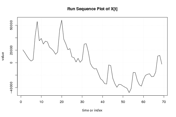
| Dataseries X: | |||||||||||||||||||||||||||||||||||||||||||||||||||||||||||||||||
20550,02 15876,62 10472,14 5741,66 2632,7 4753,38 42666,74 66105,42 35250,42 38857,54 29869,74 34522,22 33364,22 24973,22 22349,94 18776,5 13502,02 17010,18 53046,74 68228,46 37702,58 30199,38 20879,02 22549,58 9235,5 8149,5 1227,54 6985,74 655,78 4281,02 29801,14 30495,22 17511,14 -1111,86 -7026,3 -9963,34 -9582,58 -17819,34 -25724,38 -28424,86 -33549,98 -34180,74 -3575,82 -4657,42 -25043,5 -33631,98 -39363,82 -34650,9 -35115,38 -37490,06 -39324,22 -41229,1 -47991,86 -41398,38 -15573,18 -15924,98 -28571,5 -35496,54 -37603,14 -27152,02 -20334,22 -18642,22 -17761,78 -22437,02 -22103,94 -15073,86 10675,3 11603,82 -2391,82 | |||||||||||||||||||||||||||||||||||||||||||||||||||||||||||||||||
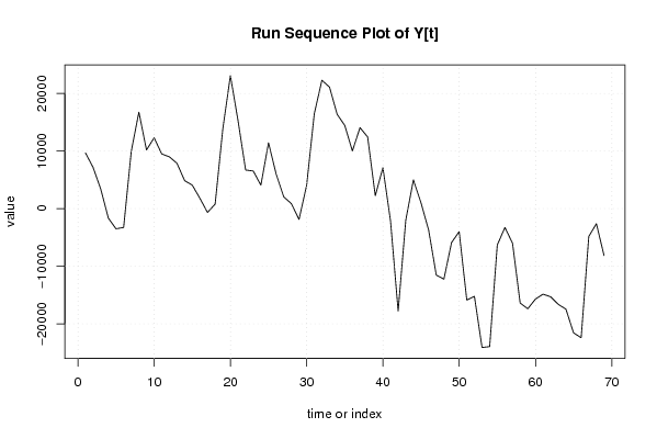
| Dataseries Y: | |||||||||||||||||||||||||||||||||||||||||||||||||||||||||||||||||
9681,09 7146,99 3398,92 -1651,65 -3500,79 -3265,17 9922,07 16760,19 10195,19 12294,52 9496,07 8991,14 7870,14 4861,39 4081,37 1797,66 -662,41 793,28 13753,32 23090,8 15300,13 6707,58 6529,84 4078,38 11434,16 6007,91 2037,02 868,07 -1878,07 4034,59 16446,17 22294,39 21096,42 16379,67 14448,21 10018,35 14059,94 12438,1 2241,99 7107,92 -2135,91 -17792,75 -2007,97 4991,63 988,41 -3731,91 -11543,47 -12240,94 -5909,26 -3994,38 -15871,07 -15220,99 -24112,08 -23953,26 -6313,71 -3272,66 -6009,34 -16395,45 -17384,1 -15708,52 -14853,57 -15305,82 -16625,61 -17450,77 -21566,55 -22416,83 -4813,14 -2620,71 -8157,22 | |||||||||||||||||||||||||||||||||||||||||||||||||||||||||||||||||
Tables (Output of Computation) | |||||||||||||||||||||||||||||||||||||||||||||||||||||||||||||||||
| |||||||||||||||||||||||||||||||||||||||||||||||||||||||||||||||||
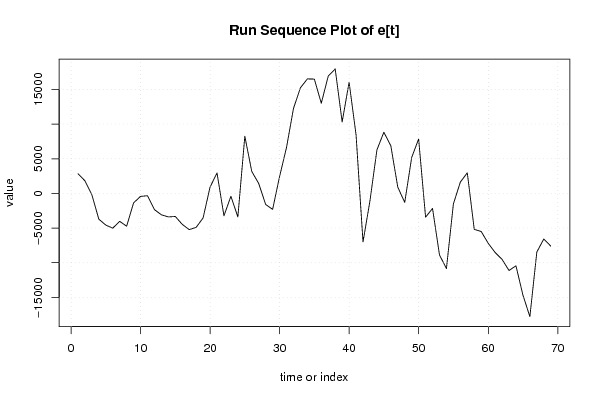
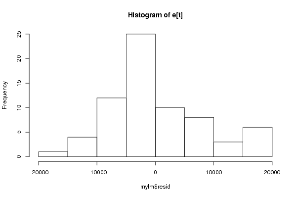
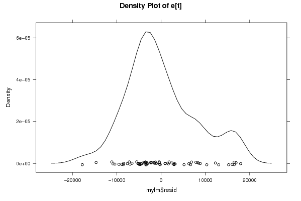
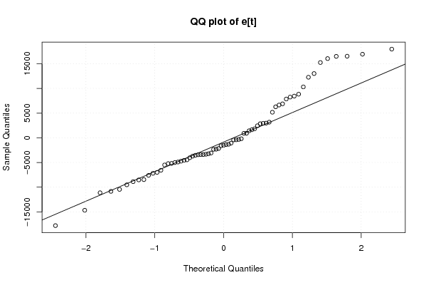
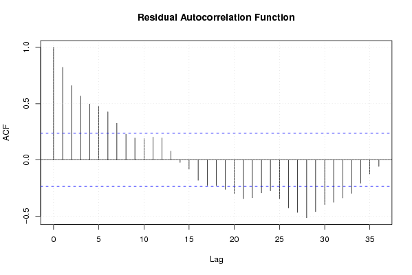
Figures (Output of Computation) | |||||||||||||||||||||||||||||||||||||||||||||||||||||||||||||||||
Input Parameters & R Code | |||||||||||||||||||||||||||||||||||||||||||||||||||||||||||||||||
| Parameters (Session): | |||||||||||||||||||||||||||||||||||||||||||||||||||||||||||||||||
| par1 = 0 ; par2 = 36 ; | |||||||||||||||||||||||||||||||||||||||||||||||||||||||||||||||||
| Parameters (R input): | |||||||||||||||||||||||||||||||||||||||||||||||||||||||||||||||||
| par1 = 0 ; par2 = 36 ; | |||||||||||||||||||||||||||||||||||||||||||||||||||||||||||||||||
| R code (references can be found in the software module): | |||||||||||||||||||||||||||||||||||||||||||||||||||||||||||||||||
par1 <- as.numeric(par1) | |||||||||||||||||||||||||||||||||||||||||||||||||||||||||||||||||