Free Statistics
of Irreproducible Research!
Description of Statistical Computation | |||||||||||||||||||||||||||||||||||||||||||||||||||||||||||||||||||||
|---|---|---|---|---|---|---|---|---|---|---|---|---|---|---|---|---|---|---|---|---|---|---|---|---|---|---|---|---|---|---|---|---|---|---|---|---|---|---|---|---|---|---|---|---|---|---|---|---|---|---|---|---|---|---|---|---|---|---|---|---|---|---|---|---|---|---|---|---|---|
| Author's title | |||||||||||||||||||||||||||||||||||||||||||||||||||||||||||||||||||||
| Author | *The author of this computation has been verified* | ||||||||||||||||||||||||||||||||||||||||||||||||||||||||||||||||||||
| R Software Module | rwasp_pairs.wasp | ||||||||||||||||||||||||||||||||||||||||||||||||||||||||||||||||||||
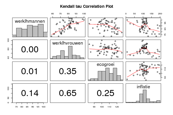
| Title produced by software | Kendall tau Correlation Matrix | ||||||||||||||||||||||||||||||||||||||||||||||||||||||||||||||||||||
| Date of computation | Fri, 06 Nov 2009 05:49:31 -0700 | ||||||||||||||||||||||||||||||||||||||||||||||||||||||||||||||||||||
| Cite this page as follows | Statistical Computations at FreeStatistics.org, Office for Research Development and Education, URL https://freestatistics.org/blog/index.php?v=date/2009/Nov/06/t1257511831420pi2kx7iy7y1x.htm/, Retrieved Sun, 28 Apr 2024 07:42:20 +0000 | ||||||||||||||||||||||||||||||||||||||||||||||||||||||||||||||||||||
| Statistical Computations at FreeStatistics.org, Office for Research Development and Education, URL https://freestatistics.org/blog/index.php?pk=54285, Retrieved Sun, 28 Apr 2024 07:42:20 +0000 | |||||||||||||||||||||||||||||||||||||||||||||||||||||||||||||||||||||
| QR Codes: | |||||||||||||||||||||||||||||||||||||||||||||||||||||||||||||||||||||
|
| |||||||||||||||||||||||||||||||||||||||||||||||||||||||||||||||||||||
| Original text written by user: | |||||||||||||||||||||||||||||||||||||||||||||||||||||||||||||||||||||
| IsPrivate? | No (this computation is public) | ||||||||||||||||||||||||||||||||||||||||||||||||||||||||||||||||||||
| User-defined keywords | ws6kendalltauindexen | ||||||||||||||||||||||||||||||||||||||||||||||||||||||||||||||||||||
| Estimated Impact | 178 | ||||||||||||||||||||||||||||||||||||||||||||||||||||||||||||||||||||
Tree of Dependent Computations | |||||||||||||||||||||||||||||||||||||||||||||||||||||||||||||||||||||
| Family? (F = Feedback message, R = changed R code, M = changed R Module, P = changed Parameters, D = changed Data) | |||||||||||||||||||||||||||||||||||||||||||||||||||||||||||||||||||||
| - [Back to Back Histogram] [3/11/2009] [2009-11-02 21:58:53] [b98453cac15ba1066b407e146608df68] - RM D [Kendall tau Correlation Matrix] [] [2009-11-06 12:49:31] [2b548c9d2e9bba6e1eaf65bd4d551f41] [Current] | |||||||||||||||||||||||||||||||||||||||||||||||||||||||||||||||||||||
| Feedback Forum | |||||||||||||||||||||||||||||||||||||||||||||||||||||||||||||||||||||
Post a new message | |||||||||||||||||||||||||||||||||||||||||||||||||||||||||||||||||||||
Dataset | |||||||||||||||||||||||||||||||||||||||||||||||||||||||||||||||||||||
| Dataseries X: | |||||||||||||||||||||||||||||||||||||||||||||||||||||||||||||||||||||
100.00 100.00 100.00 100.00 101.25 98.20 117.87 95.00 96.25 90.09 113.95 117.50 93.75 82.88 107.33 107.50 95.00 82.88 104.96 97.50 97.50 85.59 97.73 100.00 97.50 86.49 99.07 107.50 97.50 85.59 108.16 120.00 93.75 81.98 106.20 110.00 93.75 80.18 101.34 107.50 88.75 81.08 117.67 117.50 93.75 90.99 83.57 117.50 93.75 92.79 98.86 122.50 95.00 91.89 116.94 125.00 96.25 86.49 109.40 105.00 96.25 82.88 112.40 107.50 98.75 83.78 105.68 120.00 101.25 84.68 102.27 120.00 102.50 84.68 104.03 120.00 102.50 82.88 119.32 105.00 102.50 81.08 104.03 115.00 98.75 81.08 113.53 120.00 91.25 81.08 118.39 112.50 86.25 88.29 88.22 110.00 82.50 90.09 103.82 107.50 83.75 88.29 118.60 97.50 86.25 83.78 120.35 92.50 87.50 81.08 116.63 100.00 88.75 81.08 105.37 102.50 90.00 81.98 109.50 92.50 88.75 81.98 108.78 95.00 86.25 81.98 122.73 95.00 87.50 82.88 109.61 95.00 85.00 79.28 112.91 82.50 80.00 74.77 121.07 82.50 83.75 75.68 95.56 82.50 82.50 72.97 107.64 80.00 80.00 69.37 116.22 85.00 78.75 71.17 126.45 105.00 77.50 71.17 117.05 122.50 81.25 72.07 103.31 127.50 85.00 71.17 114.36 137.50 85.00 68.47 116.53 140.00 80.00 63.96 113.43 160.00 76.25 61.26 121.18 152.50 72.50 58.56 112.71 177.50 76.25 62.16 119.73 195.00 90.00 73.87 99.17 197.50 91.25 78.38 103.10 185.00 86.25 74.77 120.66 187.50 76.25 71.17 119.52 170.00 72.50 67.57 102.69 130.00 77.50 70.27 97.42 117.50 88.75 74.77 94.01 102.50 96.25 75.68 96.28 97.50 98.75 73.87 106.51 65.00 96.25 69.37 97.21 67.50 92.50 64.86 94.83 45.00 93.75 65.77 106.10 25.00 100.00 72.97 85.33 7.50 | |||||||||||||||||||||||||||||||||||||||||||||||||||||||||||||||||||||
Tables (Output of Computation) | |||||||||||||||||||||||||||||||||||||||||||||||||||||||||||||||||||||
| |||||||||||||||||||||||||||||||||||||||||||||||||||||||||||||||||||||
Figures (Output of Computation) | |||||||||||||||||||||||||||||||||||||||||||||||||||||||||||||||||||||
Input Parameters & R Code | |||||||||||||||||||||||||||||||||||||||||||||||||||||||||||||||||||||
| Parameters (Session): | |||||||||||||||||||||||||||||||||||||||||||||||||||||||||||||||||||||
| Parameters (R input): | |||||||||||||||||||||||||||||||||||||||||||||||||||||||||||||||||||||
| R code (references can be found in the software module): | |||||||||||||||||||||||||||||||||||||||||||||||||||||||||||||||||||||
panel.tau <- function(x, y, digits=2, prefix='', cex.cor) | |||||||||||||||||||||||||||||||||||||||||||||||||||||||||||||||||||||