Free Statistics
of Irreproducible Research!
Description of Statistical Computation | |||||||||||||||||||||
|---|---|---|---|---|---|---|---|---|---|---|---|---|---|---|---|---|---|---|---|---|---|
| Author's title | |||||||||||||||||||||
| Author | *The author of this computation has been verified* | ||||||||||||||||||||
| R Software Module | rwasp_cloud.wasp | ||||||||||||||||||||
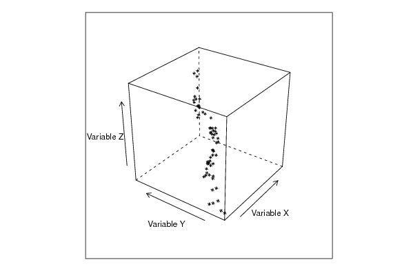
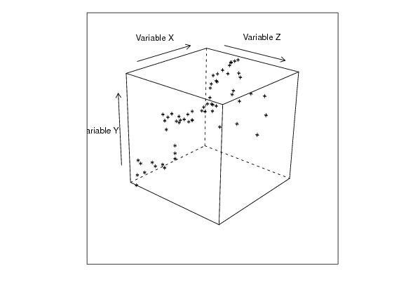
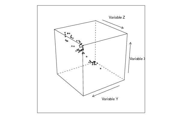
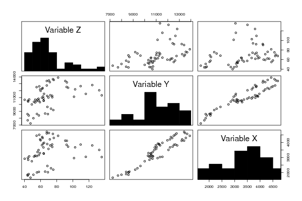
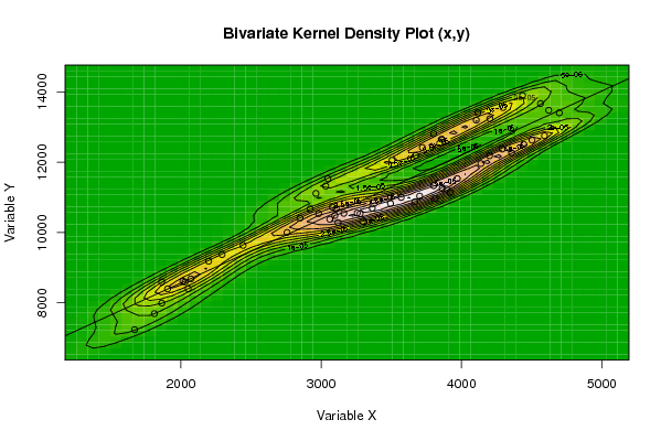
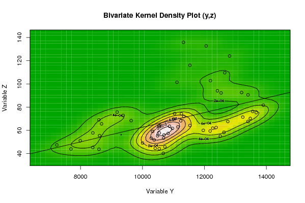
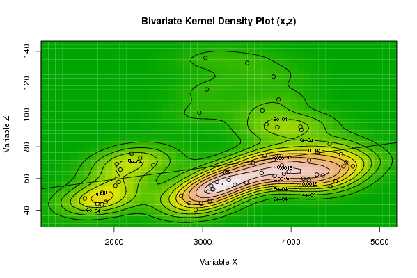
| Title produced by software | Trivariate Scatterplots | ||||||||||||||||||||
| Date of computation | Fri, 06 Nov 2009 07:09:53 -0700 | ||||||||||||||||||||
| Cite this page as follows | Statistical Computations at FreeStatistics.org, Office for Research Development and Education, URL https://freestatistics.org/blog/index.php?v=date/2009/Nov/06/t1257516619wrv0ixipg5wlfng.htm/, Retrieved Sun, 28 Apr 2024 00:59:46 +0000 | ||||||||||||||||||||
| Statistical Computations at FreeStatistics.org, Office for Research Development and Education, URL https://freestatistics.org/blog/index.php?pk=54317, Retrieved Sun, 28 Apr 2024 00:59:46 +0000 | |||||||||||||||||||||
| QR Codes: | |||||||||||||||||||||
|
| |||||||||||||||||||||
| Original text written by user: | |||||||||||||||||||||
| IsPrivate? | No (this computation is public) | ||||||||||||||||||||
| User-defined keywords | |||||||||||||||||||||
| Estimated Impact | 127 | ||||||||||||||||||||
Tree of Dependent Computations | |||||||||||||||||||||
| Family? (F = Feedback message, R = changed R code, M = changed R Module, P = changed Parameters, D = changed Data) | |||||||||||||||||||||
| - [Bivariate Explorative Data Analysis] [WS4 part 2] [2009-11-03 21:24:08] [f15cf5036ae52d4243ad71d4fb151dbe] - RMPD [Trivariate Scatterplots] [WS5 part 2] [2009-11-06 14:09:53] [1aecede37375310a889a187dca5e5c0a] [Current] - P [Trivariate Scatterplots] [Ws5 part 2] [2009-11-06 14:13:31] [f15cf5036ae52d4243ad71d4fb151dbe] - RMP [Partial Correlation] [WS5 part 3] [2009-11-06 14:22:23] [f15cf5036ae52d4243ad71d4fb151dbe] - [Partial Correlation] [dqsfqdsf] [2010-11-18 12:59:02] [f15cf5036ae52d4243ad71d4fb151dbe] | |||||||||||||||||||||
| Feedback Forum | |||||||||||||||||||||
Post a new message | |||||||||||||||||||||
Dataset | |||||||||||||||||||||
| Dataseries X: | |||||||||||||||||||||
2756.76 2849.27 2921.44 2981.85 3080.58 3106.22 3119.31 3061.26 3097.31 3161.69 3257.16 3277.01 3295.32 3363.99 3494.17 3667.03 3813.06 3917.96 3895.51 3801.06 3570.12 3701.61 3862.27 3970.10 4138.52 4199.75 4290.89 4443.91 4502.64 4356.98 4591.27 4696.96 4621.40 4562.84 4202.52 4296.49 4435.23 4105.18 4116.68 3844.49 3720.98 3674.40 3857.62 3801.06 3504.37 3032.60 3047.03 2962.34 2197.82 2014.45 1862.83 1905.41 1810.99 1670.07 1864.44 2052.02 2029.60 2070.83 2293.41 2443.27 | |||||||||||||||||||||
| Dataseries Y: | |||||||||||||||||||||
10001.60 10411.75 10673.38 10539.51 10723.78 10682.06 10283.19 10377.18 10486.64 10545.38 10554.27 10532.54 10324.31 10695.25 10827.81 10872.48 10971.19 11145.65 11234.68 11333.88 10997.97 11036.89 11257.35 11533.59 11963.12 12185.15 12377.62 12512.89 12631.48 12268.53 12754.80 13407.75 13480.21 13673.28 13239.71 13557.69 13901.28 13200.58 13406.97 12538.12 12419.57 12193.88 12656.63 12812.48 12056.67 11322.38 11530.75 11114.08 9181.73 8614.55 8595.56 8396.20 7690.50 7235.47 7992.12 8398.37 8593.01 8679.75 9374.63 9634.97 | |||||||||||||||||||||
| Dataseries Z: | |||||||||||||||||||||
49.14 44.61 40.22 44.23 45.85 53.38 53.26 51.8 55.3 57.81 63.96 63.77 59.15 56.12 57.42 63.52 61.71 63.01 68.18 72.03 69.75 74.41 74.33 64.24 60.03 59.44 62.5 55.04 58.34 61.92 67.65 67.68 70.3 75.26 71.44 76.36 81.71 92.6 90.6 92.23 94.09 102.79 109.65 124.05 132.69 135.81 116.07 101.42 75.73 55.48 43.8 45.29 44.01 47.48 51.07 57.84 69.04 65.61 72.87 68.41 | |||||||||||||||||||||
Tables (Output of Computation) | |||||||||||||||||||||
| |||||||||||||||||||||
Figures (Output of Computation) | |||||||||||||||||||||
Input Parameters & R Code | |||||||||||||||||||||
| Parameters (Session): | |||||||||||||||||||||
| par1 = 50 ; par2 = 50 ; par3 = Y ; par4 = Y ; par5 = Variable X ; par6 = Variable Y ; par7 = Variable Z ; | |||||||||||||||||||||
| Parameters (R input): | |||||||||||||||||||||
| par1 = 50 ; par2 = 50 ; par3 = Y ; par4 = Y ; par5 = Variable X ; par6 = Variable Y ; par7 = Variable Z ; | |||||||||||||||||||||
| R code (references can be found in the software module): | |||||||||||||||||||||
x <- array(x,dim=c(length(x),1)) | |||||||||||||||||||||