Free Statistics
of Irreproducible Research!
Description of Statistical Computation | |||||||||||||||||||||
|---|---|---|---|---|---|---|---|---|---|---|---|---|---|---|---|---|---|---|---|---|---|
| Author's title | |||||||||||||||||||||
| Author | *The author of this computation has been verified* | ||||||||||||||||||||
| R Software Module | rwasp_sdplot.wasp | ||||||||||||||||||||
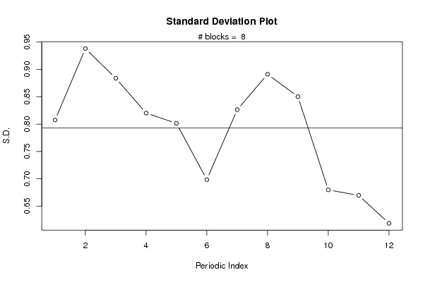
| Title produced by software | Standard Deviation Plot | ||||||||||||||||||||
| Date of computation | Sun, 08 Nov 2009 09:22:41 -0700 | ||||||||||||||||||||
| Cite this page as follows | Statistical Computations at FreeStatistics.org, Office for Research Development and Education, URL https://freestatistics.org/blog/index.php?v=date/2009/Nov/08/t1257697408oobchp5d7sl3jqz.htm/, Retrieved Sat, 04 May 2024 10:47:47 +0000 | ||||||||||||||||||||
| Statistical Computations at FreeStatistics.org, Office for Research Development and Education, URL https://freestatistics.org/blog/index.php?pk=54601, Retrieved Sat, 04 May 2024 10:47:47 +0000 | |||||||||||||||||||||
| QR Codes: | |||||||||||||||||||||
|
| |||||||||||||||||||||
| Original text written by user: | |||||||||||||||||||||
| IsPrivate? | No (this computation is public) | ||||||||||||||||||||
| User-defined keywords | ws6multi12 | ||||||||||||||||||||
| Estimated Impact | 170 | ||||||||||||||||||||
Tree of Dependent Computations | |||||||||||||||||||||
| Family? (F = Feedback message, R = changed R code, M = changed R Module, P = changed Parameters, D = changed Data) | |||||||||||||||||||||
| - [Standard Deviation Plot] [3/11/2009] [2009-11-02 22:09:58] [b98453cac15ba1066b407e146608df68] F PD [Standard Deviation Plot] [] [2009-11-08 16:22:41] [42ed2e0ab6f351a3dce7cf3f388e378d] [Current] | |||||||||||||||||||||
| Feedback Forum | |||||||||||||||||||||
Post a new message | |||||||||||||||||||||
Dataset | |||||||||||||||||||||
| Dataseries X: | |||||||||||||||||||||
6,3 6,1 6,1 6,3 6,3 6 6,2 6,4 6,8 7,5 7,5 7,6 7,6 7,4 7,3 7,1 6,9 6,8 7,5 7,6 7,8 8 8,1 8,2 8,3 8,2 8 7,9 7,6 7,6 8,3 8,4 8,4 8,4 8,4 8,6 8,9 8,8 8,3 7,5 7,2 7,4 8,8 9,3 9,3 8,7 8,2 8,3 8,5 8,6 8,5 8,2 8,1 7,9 8,6 8,7 8,7 8,5 8,4 8,5 8,7 8,7 8,6 8,5 8,3 8 8,2 8,1 8,1 8 7,9 7,9 8 8 7,9 8 7,7 7,2 7,5 7,3 7 7 7 7,2 7,3 7,1 6,8 6,4 6,1 6,5 7,7 7,9 7,5 6,9 6,6 6,9 7,7 | |||||||||||||||||||||
Tables (Output of Computation) | |||||||||||||||||||||
| |||||||||||||||||||||
Figures (Output of Computation) | |||||||||||||||||||||
Input Parameters & R Code | |||||||||||||||||||||
| Parameters (Session): | |||||||||||||||||||||
| par1 = 12 ; | |||||||||||||||||||||
| Parameters (R input): | |||||||||||||||||||||
| par1 = 12 ; | |||||||||||||||||||||
| R code (references can be found in the software module): | |||||||||||||||||||||
par1 <- as.numeric(par1) | |||||||||||||||||||||