Free Statistics
of Irreproducible Research!
Description of Statistical Computation | |||||||||||||||||||||
|---|---|---|---|---|---|---|---|---|---|---|---|---|---|---|---|---|---|---|---|---|---|
| Author's title | |||||||||||||||||||||
| Author | *The author of this computation has been verified* | ||||||||||||||||||||
| R Software Module | rwasp_cloud.wasp | ||||||||||||||||||||
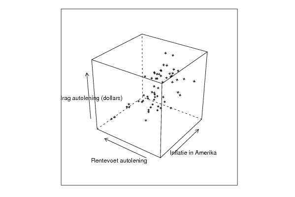
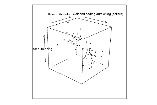
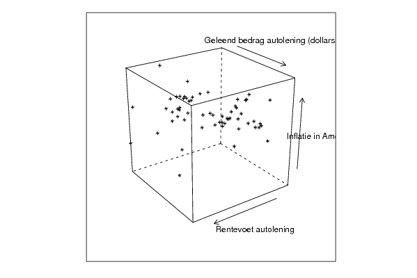
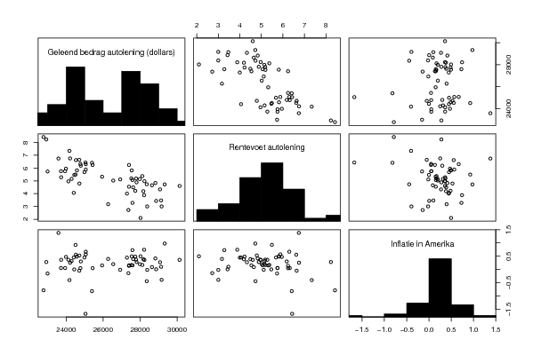
| Title produced by software | Trivariate Scatterplots | ||||||||||||||||||||
| Date of computation | Mon, 09 Nov 2009 12:22:48 -0700 | ||||||||||||||||||||
| Cite this page as follows | Statistical Computations at FreeStatistics.org, Office for Research Development and Education, URL https://freestatistics.org/blog/index.php?v=date/2009/Nov/09/t12577946733vm00i6loh27kgb.htm/, Retrieved Sat, 05 Jul 2025 20:44:45 +0000 | ||||||||||||||||||||
| Statistical Computations at FreeStatistics.org, Office for Research Development and Education, URL https://freestatistics.org/blog/index.php?pk=54939, Retrieved Sat, 05 Jul 2025 20:44:45 +0000 | |||||||||||||||||||||
| QR Codes: | |||||||||||||||||||||
|
| |||||||||||||||||||||
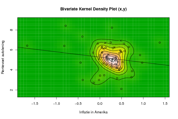
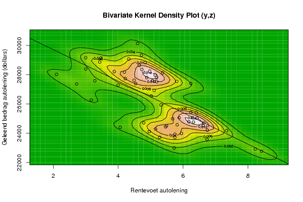
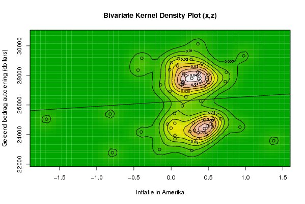
| Original text written by user: | Inflatie in Amerika, Rentevoet autolening en geleend bedrag autolening | ||||||||||||||||||||
| IsPrivate? | No (this computation is public) | ||||||||||||||||||||
| User-defined keywords | |||||||||||||||||||||
| Estimated Impact | 225 | ||||||||||||||||||||
Tree of Dependent Computations | |||||||||||||||||||||
| Family? (F = Feedback message, R = changed R code, M = changed R Module, P = changed Parameters, D = changed Data) | |||||||||||||||||||||
| - [Box-Cox Linearity Plot] [3/11/2009] [2009-11-02 21:47:57] [b98453cac15ba1066b407e146608df68] - RMPD [Trivariate Scatterplots] [shw5: Trivariate ...] [2009-11-09 19:22:48] [7a39e26d7a09dd77604df90cb29f8d39] [Current] | |||||||||||||||||||||
| Feedback Forum | |||||||||||||||||||||
Post a new message | |||||||||||||||||||||
Dataset | |||||||||||||||||||||
| Dataseries X: | |||||||||||||||||||||
0.527 0.472 0.000 0.052 0.313 0.364 0.363 -0.155 0.052 0.568 0.668 1.378 0.252 -0.402 -0.050 0.555 0.050 0.150 0.450 0.299 0.199 0.496 0.444 -0.393 -0.444 0.198 0.494 0.133 0.388 0.484 0.278 0.369 0.165 0.155 0.087 0.414 0.360 0.975 0.270 0.359 0.169 0.381 0.154 0.486 0.925 0.728 -0.014 0.046 -0.819 -1.674 -0.788 0.279 0.396 -0.141 -0.019 0.099 0.742 0.005 0.448 | |||||||||||||||||||||
| Dataseries Y: | |||||||||||||||||||||
4.79 5.95 5.46 5.75 5.15 4.96 5.28 5.73 5.75 5.88 6.3 6.74 6.75 7.34 6.64 6.62 6.32 5.32 5.68 6.18 5.02 2.1 4 3 4.73 5.14 5.81 6.24 4.49 4.22 4.88 5.18 5.19 5.06 4.65 4.83 4.6 4.72 4.33 4.97 5.37 4.19 4.54 5.82 5.49 3.28 5.11 6.24 6.41 6.43 8.42 8.23 3.17 2.72 3 3.47 3.88 3.43 4.06 | |||||||||||||||||||||
| Dataseries Z: | |||||||||||||||||||||
24710.92 23983.59 24434.12 23939.23 24290.02 24117.63 23724.64 22989.44 23716.86 25058.83 25059.00 23579.18 24209.03 24173.67 24706.39 24522.12 24766.15 25940.04 24985.78 24788.00 26544.56 28019.08 27285.71 29161.16 28357.73 27979.91 27543.95 27397.53 27623.59 27736.07 27803.79 27779.55 27524.13 27582.72 28638.95 28825.78 30132.61 29326.85 29075.62 28230.63 28118.36 28173.29 27396.91 24578.55 24504.77 27582.37 26920.31 25426.68 25390.80 25041.16 22769.42 22921.89 26267.63 27364.67 28382.59 29132.81 28214.51 28865.73 24405.35 | |||||||||||||||||||||
Tables (Output of Computation) | |||||||||||||||||||||
| |||||||||||||||||||||
Figures (Output of Computation) | |||||||||||||||||||||
Input Parameters & R Code | |||||||||||||||||||||
| Parameters (Session): | |||||||||||||||||||||
| par1 = 50 ; par2 = 50 ; par3 = Y ; par4 = Y ; par5 = Inflatie in Amerika ; par6 = Rentevoet autolening ; par7 = Geleend bedrag autolening (dollars) ; | |||||||||||||||||||||
| Parameters (R input): | |||||||||||||||||||||
| par1 = 50 ; par2 = 50 ; par3 = Y ; par4 = Y ; par5 = Inflatie in Amerika ; par6 = Rentevoet autolening ; par7 = Geleend bedrag autolening (dollars) ; | |||||||||||||||||||||
| R code (references can be found in the software module): | |||||||||||||||||||||
x <- array(x,dim=c(length(x),1)) | |||||||||||||||||||||