Free Statistics
of Irreproducible Research!
Description of Statistical Computation | |||||||||||||||||||||
|---|---|---|---|---|---|---|---|---|---|---|---|---|---|---|---|---|---|---|---|---|---|
| Author's title | |||||||||||||||||||||
| Author | *The author of this computation has been verified* | ||||||||||||||||||||
| R Software Module | rwasp_meanplot.wasp | ||||||||||||||||||||
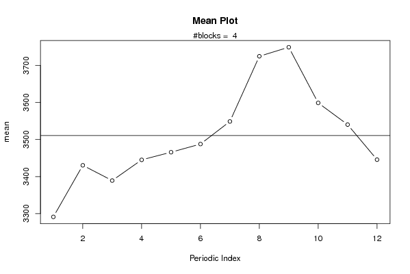
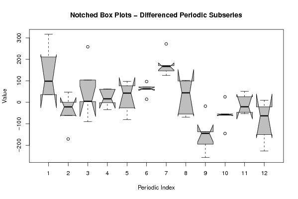
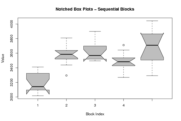
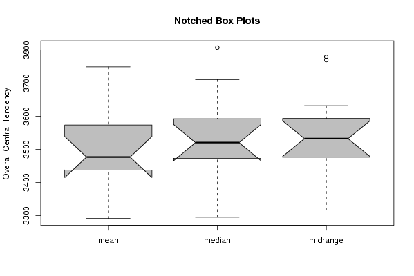
| Title produced by software | Mean Plot | ||||||||||||||||||||
| Date of computation | Fri, 13 Nov 2009 16:46:28 -0700 | ||||||||||||||||||||
| Cite this page as follows | Statistical Computations at FreeStatistics.org, Office for Research Development and Education, URL https://freestatistics.org/blog/index.php?v=date/2009/Nov/14/t12581560592tf5i3dwgcl5ibl.htm/, Retrieved Sun, 28 Apr 2024 13:37:59 +0000 | ||||||||||||||||||||
| Statistical Computations at FreeStatistics.org, Office for Research Development and Education, URL https://freestatistics.org/blog/index.php?pk=57189, Retrieved Sun, 28 Apr 2024 13:37:59 +0000 | |||||||||||||||||||||
| QR Codes: | |||||||||||||||||||||
|
| |||||||||||||||||||||
| Original text written by user: | |||||||||||||||||||||
| IsPrivate? | No (this computation is public) | ||||||||||||||||||||
| User-defined keywords | |||||||||||||||||||||
| Estimated Impact | 235 | ||||||||||||||||||||
Tree of Dependent Computations | |||||||||||||||||||||
| Family? (F = Feedback message, R = changed R code, M = changed R Module, P = changed Parameters, D = changed Data) | |||||||||||||||||||||
| - [Bagplot] [3/11/2009] [2009-11-02 21:51:11] [b98453cac15ba1066b407e146608df68] - PD [Bagplot] [Bagplot icv en icg] [2009-11-09 10:21:28] [134dc66689e3d457a82860db6471d419] - RMPD [Mean Plot] [Mean plot Yt] [2009-11-13 23:46:28] [b243db81ea3e1f02fb3382887fb0f701] [Current] | |||||||||||||||||||||
| Feedback Forum | |||||||||||||||||||||
Post a new message | |||||||||||||||||||||
Dataset | |||||||||||||||||||||
| Dataseries X: | |||||||||||||||||||||
3016.70 3052.40 3099.60 3103.30 3119.80 3093.70 3164.90 3311.50 3410.60 3392.60 3338.20 3285.10 3294.80 3611.20 3611.30 3521.00 3519.30 3438.30 3534.90 3705.80 3807.60 3663.00 3604.50 3563.80 3511.40 3546.50 3525.40 3529.90 3591.60 3668.30 3728.80 3853.60 3897.70 3640.70 3495.50 3495.10 3268.00 3479.10 3417.80 3521.30 3487.10 3529.90 3544.30 3710.80 3641.90 3447.10 3386.80 3438.50 3364.30 3462.70 3291.90 3550.00 3611.00 3708.60 3771.10 4042.70 3988.40 3851.20 3876.70 | |||||||||||||||||||||
Tables (Output of Computation) | |||||||||||||||||||||
| |||||||||||||||||||||
Figures (Output of Computation) | |||||||||||||||||||||
Input Parameters & R Code | |||||||||||||||||||||
| Parameters (Session): | |||||||||||||||||||||
| par1 = 12 ; | |||||||||||||||||||||
| Parameters (R input): | |||||||||||||||||||||
| par1 = 12 ; | |||||||||||||||||||||
| R code (references can be found in the software module): | |||||||||||||||||||||
par1 <- as.numeric(par1) | |||||||||||||||||||||