Free Statistics
of Irreproducible Research!
Description of Statistical Computation | |||||||||||||||||||||
|---|---|---|---|---|---|---|---|---|---|---|---|---|---|---|---|---|---|---|---|---|---|
| Author's title | |||||||||||||||||||||
| Author | *The author of this computation has been verified* | ||||||||||||||||||||
| R Software Module | rwasp_meanplot.wasp | ||||||||||||||||||||
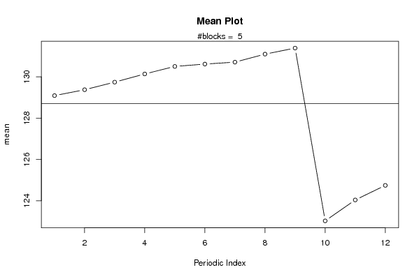
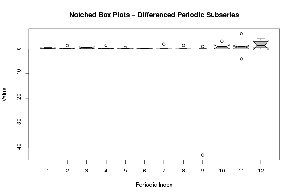
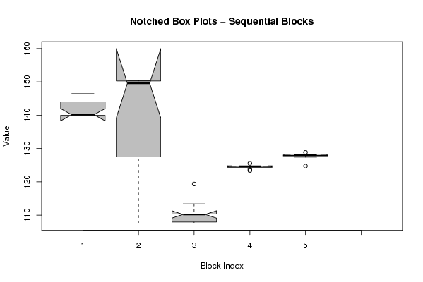
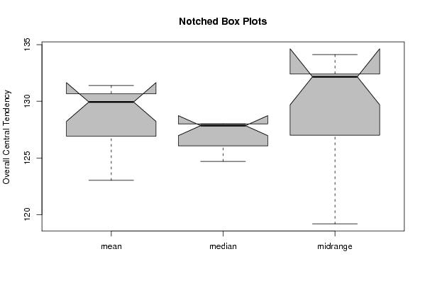
| Title produced by software | Mean Plot | ||||||||||||||||||||
| Date of computation | Fri, 13 Nov 2009 18:21:17 -0700 | ||||||||||||||||||||
| Cite this page as follows | Statistical Computations at FreeStatistics.org, Office for Research Development and Education, URL https://freestatistics.org/blog/index.php?v=date/2009/Nov/14/t12581617724xvqjvbuwkqcp0g.htm/, Retrieved Sat, 27 Apr 2024 23:18:29 +0000 | ||||||||||||||||||||
| Statistical Computations at FreeStatistics.org, Office for Research Development and Education, URL https://freestatistics.org/blog/index.php?pk=57207, Retrieved Sat, 27 Apr 2024 23:18:29 +0000 | |||||||||||||||||||||
| QR Codes: | |||||||||||||||||||||
|
| |||||||||||||||||||||
| Original text written by user: | |||||||||||||||||||||
| IsPrivate? | No (this computation is public) | ||||||||||||||||||||
| User-defined keywords | |||||||||||||||||||||
| Estimated Impact | 212 | ||||||||||||||||||||
Tree of Dependent Computations | |||||||||||||||||||||
| Family? (F = Feedback message, R = changed R code, M = changed R Module, P = changed Parameters, D = changed Data) | |||||||||||||||||||||
| - [Back to Back Histogram] [3/11/2009] [2009-11-02 21:58:53] [b98453cac15ba1066b407e146608df68] - RMPD [Mean Plot] [] [2009-11-14 01:21:17] [dd88bf4749af0c195ad4f54cb428da1c] [Current] | |||||||||||||||||||||
| Feedback Forum | |||||||||||||||||||||
Post a new message | |||||||||||||||||||||
Dataset | |||||||||||||||||||||
| Dataseries X: | |||||||||||||||||||||
139,72 139,91 139,97 139,98 140,03 140,03 140,26 142,15 143,54 144,5 145,65 146,47 147,36 147,89 149,23 149,93 150,24 150,15 150,31 150,31 150,37 107,59 107,59 107,59 107,59 107,59 107,58 108,28 109,71 110,21 110,27 110,32 110,33 110,33 113,38 119,37 123,37 123,75 124,13 124,59 124,59 124,68 124,7 124,7 124,7 124,7 124,71 125,55 127,41 127,73 127,8 127,91 127,94 128,01 128,01 128,01 128,01 128,01 128,86 124,74 | |||||||||||||||||||||
Tables (Output of Computation) | |||||||||||||||||||||
| |||||||||||||||||||||
Figures (Output of Computation) | |||||||||||||||||||||
Input Parameters & R Code | |||||||||||||||||||||
| Parameters (Session): | |||||||||||||||||||||
| par1 = red ; par2 = blue ; par3 = TRUE ; par4 = iptot ; par5 = ipkl ; | |||||||||||||||||||||
| Parameters (R input): | |||||||||||||||||||||
| par1 = 12 ; | |||||||||||||||||||||
| R code (references can be found in the software module): | |||||||||||||||||||||
par1 <- as.numeric(par1) | |||||||||||||||||||||