Free Statistics
of Irreproducible Research!
Description of Statistical Computation | |||||||||||||||||||||||||||||||||||||||||||||
|---|---|---|---|---|---|---|---|---|---|---|---|---|---|---|---|---|---|---|---|---|---|---|---|---|---|---|---|---|---|---|---|---|---|---|---|---|---|---|---|---|---|---|---|---|---|
| Author's title | |||||||||||||||||||||||||||||||||||||||||||||
| Author | *The author of this computation has been verified* | ||||||||||||||||||||||||||||||||||||||||||||
| R Software Module | rwasp_boxcoxlin.wasp | ||||||||||||||||||||||||||||||||||||||||||||
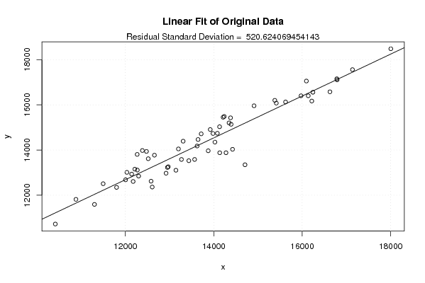
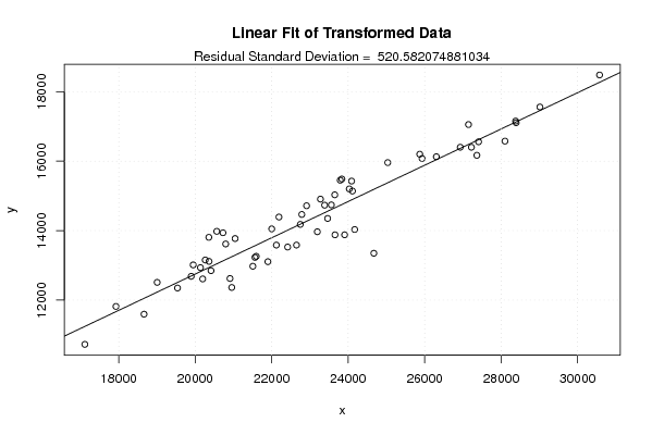
| Title produced by software | Box-Cox Linearity Plot | ||||||||||||||||||||||||||||||||||||||||||||
| Date of computation | Sat, 14 Nov 2009 08:20:55 -0700 | ||||||||||||||||||||||||||||||||||||||||||||
| Cite this page as follows | Statistical Computations at FreeStatistics.org, Office for Research Development and Education, URL https://freestatistics.org/blog/index.php?v=date/2009/Nov/14/t1258212244oh75fgg0yjtgv7i.htm/, Retrieved Sat, 27 Apr 2024 18:37:53 +0000 | ||||||||||||||||||||||||||||||||||||||||||||
| Statistical Computations at FreeStatistics.org, Office for Research Development and Education, URL https://freestatistics.org/blog/index.php?pk=57237, Retrieved Sat, 27 Apr 2024 18:37:53 +0000 | |||||||||||||||||||||||||||||||||||||||||||||
| QR Codes: | |||||||||||||||||||||||||||||||||||||||||||||
|
| |||||||||||||||||||||||||||||||||||||||||||||
| Original text written by user: | |||||||||||||||||||||||||||||||||||||||||||||
| IsPrivate? | No (this computation is public) | ||||||||||||||||||||||||||||||||||||||||||||
| User-defined keywords | |||||||||||||||||||||||||||||||||||||||||||||
| Estimated Impact | 142 | ||||||||||||||||||||||||||||||||||||||||||||
Tree of Dependent Computations | |||||||||||||||||||||||||||||||||||||||||||||
| Family? (F = Feedback message, R = changed R code, M = changed R Module, P = changed Parameters, D = changed Data) | |||||||||||||||||||||||||||||||||||||||||||||
| - [Box-Cox Linearity Plot] [3/11/2009] [2009-11-02 21:47:57] [b98453cac15ba1066b407e146608df68] - D [Box-Cox Linearity Plot] [WS6] [2009-11-14 15:20:55] [48076ccf082563ab8a2c81e57fdb5364] [Current] | |||||||||||||||||||||||||||||||||||||||||||||
| Feedback Forum | |||||||||||||||||||||||||||||||||||||||||||||
Post a new message | |||||||||||||||||||||||||||||||||||||||||||||
Dataset | |||||||||||||||||||||||||||||||||||||||||||||
| Dataseries X: | |||||||||||||||||||||||||||||||||||||||||||||
10414,9 12476,8 12384,6 12266,7 12919,9 11497,3 12142 13919,4 12656,8 12034,1 13199,7 10881,3 11301,2 13643,9 12517 13981,1 14275,7 13435 13565,7 16216,3 12970 14079,9 14235 12213,4 12581 14130,4 14210,8 14378,5 13142,8 13714,7 13621,9 15379,8 13306,3 14391,2 14909,9 14025,4 12951,2 14344,3 16093,4 15413,6 14705,7 15972,8 16241,4 16626,4 17136,2 15622,9 18003,9 16136,1 14423,7 16789,4 16782,2 14133,8 12607 12004,5 12175,4 13268 12299,3 11800,6 13873,3 12269,6 | |||||||||||||||||||||||||||||||||||||||||||||
| Dataseries Y: | |||||||||||||||||||||||||||||||||||||||||||||
10723,8 13938,9 13979,8 13807,4 12973,9 12509,8 12934,1 14908,3 13772,1 13012,6 14049,9 11816,5 11593,2 14466,2 13615,9 14733,9 13880,7 13527,5 13584 16170,2 13260,6 14741,9 15486,5 13154,5 12621,2 15031,6 15452,4 15428 13105,9 14716,8 14180 16202,2 14392,4 15140,6 15960,1 14351,3 13230,2 15202,1 17056 16077,7 13348,2 16402,4 16559,1 16579 17561,2 16129,6 18484,3 16402,6 14032,3 17109,1 17157,2 13879,8 12362,4 12683,5 12608,8 13583,7 12846,3 12347,1 13967 13114,3 | |||||||||||||||||||||||||||||||||||||||||||||
Tables (Output of Computation) | |||||||||||||||||||||||||||||||||||||||||||||
| |||||||||||||||||||||||||||||||||||||||||||||
Figures (Output of Computation) | |||||||||||||||||||||||||||||||||||||||||||||
Input Parameters & R Code | |||||||||||||||||||||||||||||||||||||||||||||
| Parameters (Session): | |||||||||||||||||||||||||||||||||||||||||||||
| Parameters (R input): | |||||||||||||||||||||||||||||||||||||||||||||
| R code (references can be found in the software module): | |||||||||||||||||||||||||||||||||||||||||||||
n <- length(x) | |||||||||||||||||||||||||||||||||||||||||||||