Free Statistics
of Irreproducible Research!
Description of Statistical Computation | |||||||||||||||||||||||||||||||||||||||||||||||||||||
|---|---|---|---|---|---|---|---|---|---|---|---|---|---|---|---|---|---|---|---|---|---|---|---|---|---|---|---|---|---|---|---|---|---|---|---|---|---|---|---|---|---|---|---|---|---|---|---|---|---|---|---|---|---|
| Author's title | |||||||||||||||||||||||||||||||||||||||||||||||||||||
| Author | *The author of this computation has been verified* | ||||||||||||||||||||||||||||||||||||||||||||||||||||
| R Software Module | rwasp_edauni.wasp | ||||||||||||||||||||||||||||||||||||||||||||||||||||
| Title produced by software | Univariate Explorative Data Analysis | ||||||||||||||||||||||||||||||||||||||||||||||||||||
| Date of computation | Sat, 14 Nov 2009 08:26:06 -0700 | ||||||||||||||||||||||||||||||||||||||||||||||||||||
| Cite this page as follows | Statistical Computations at FreeStatistics.org, Office for Research Development and Education, URL https://freestatistics.org/blog/index.php?v=date/2009/Nov/14/t1258212507svt158swceiyq6t.htm/, Retrieved Sun, 28 Apr 2024 03:48:47 +0000 | ||||||||||||||||||||||||||||||||||||||||||||||||||||
| Statistical Computations at FreeStatistics.org, Office for Research Development and Education, URL https://freestatistics.org/blog/index.php?pk=57239, Retrieved Sun, 28 Apr 2024 03:48:47 +0000 | |||||||||||||||||||||||||||||||||||||||||||||||||||||
| QR Codes: | |||||||||||||||||||||||||||||||||||||||||||||||||||||
|
| |||||||||||||||||||||||||||||||||||||||||||||||||||||
| Original text written by user: | |||||||||||||||||||||||||||||||||||||||||||||||||||||
| IsPrivate? | No (this computation is public) | ||||||||||||||||||||||||||||||||||||||||||||||||||||
| User-defined keywords | |||||||||||||||||||||||||||||||||||||||||||||||||||||
| Estimated Impact | 174 | ||||||||||||||||||||||||||||||||||||||||||||||||||||
Tree of Dependent Computations | |||||||||||||||||||||||||||||||||||||||||||||||||||||
| Family? (F = Feedback message, R = changed R code, M = changed R Module, P = changed Parameters, D = changed Data) | |||||||||||||||||||||||||||||||||||||||||||||||||||||
| - [Central Tendency] [SHW_WS3_Yt=c+Xt] [2009-10-16 08:10:06] [8b1aef4e7013bd33fbc2a5833375c5f5] - RMPD [Univariate Explorative Data Analysis] [] [2009-11-02 10:43:25] [8b1aef4e7013bd33fbc2a5833375c5f5] - D [Univariate Explorative Data Analysis] [ws 3] [2009-11-14 15:26:06] [f7d3e79b917995ba1c8c80042fc22ef9] [Current] | |||||||||||||||||||||||||||||||||||||||||||||||||||||
| Feedback Forum | |||||||||||||||||||||||||||||||||||||||||||||||||||||
Post a new message | |||||||||||||||||||||||||||||||||||||||||||||||||||||
Dataset | |||||||||||||||||||||||||||||||||||||||||||||||||||||
| Dataseries X: | |||||||||||||||||||||||||||||||||||||||||||||||||||||
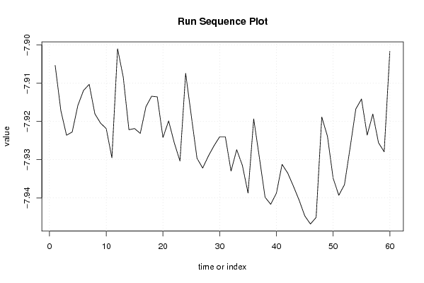
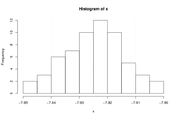
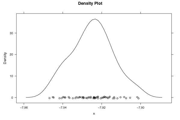
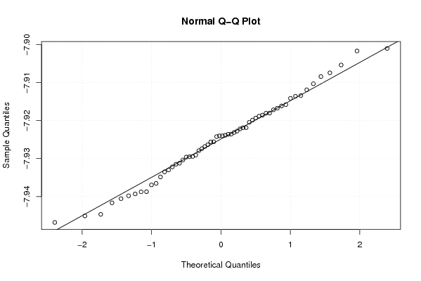
-7,905391658 -7,917186109 -7,923617208 -7,922787194 -7,915821501 -7,911917098 -7,910323253 -7,918032787 -7,920465567 -7,921890068 -7,929527208 -7,901035673 -7,908421053 -7,922182469 -7,921875 -7,923147301 -7,91617357 -7,913432836 -7,913604767 -7,924229075 -7,919886899 -7,92562724 -7,930374238 -7,90744921 -7,918592965 -7,929626412 -7,93220339 -7,929084381 -7,926374651 -7,924026591 -7,924026591 -7,932994063 -7,927404719 -7,931494662 -7,938723404 -7,919354839 -7,929468599 -7,939810834 -7,941666667 -7,938757655 -7,931232092 -7,933515483 -7,936944938 -7,940559441 -7,944684529 -7,946817786 -7,945101351 -7,91886196 -7,9238921 -7,93483927 -7,939313984 -7,936538462 -7,926829268 -7,916756757 -7,91416309 -7,923591213 -7,918085106 -7,925586137 -7,927945472 -7,901699029 | |||||||||||||||||||||||||||||||||||||||||||||||||||||
Tables (Output of Computation) | |||||||||||||||||||||||||||||||||||||||||||||||||||||
| |||||||||||||||||||||||||||||||||||||||||||||||||||||
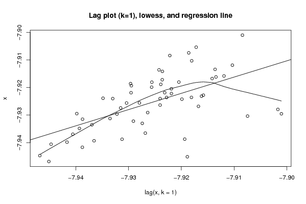
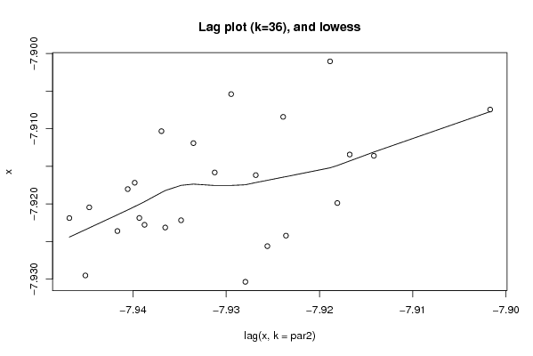
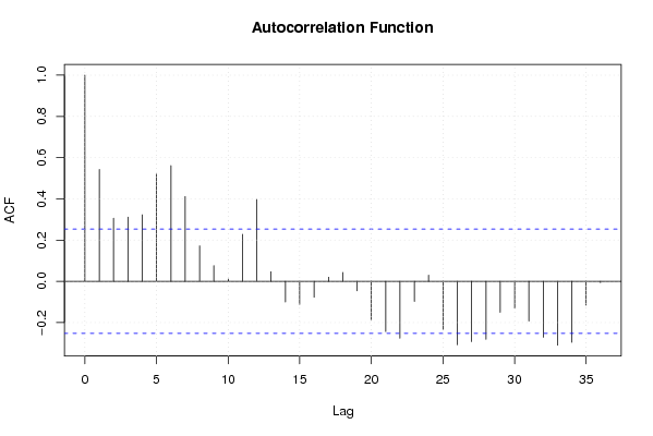
Figures (Output of Computation) | |||||||||||||||||||||||||||||||||||||||||||||||||||||
Input Parameters & R Code | |||||||||||||||||||||||||||||||||||||||||||||||||||||
| Parameters (Session): | |||||||||||||||||||||||||||||||||||||||||||||||||||||
| par1 = 0 ; par2 = 36 ; | |||||||||||||||||||||||||||||||||||||||||||||||||||||
| Parameters (R input): | |||||||||||||||||||||||||||||||||||||||||||||||||||||
| par1 = 0 ; par2 = 36 ; | |||||||||||||||||||||||||||||||||||||||||||||||||||||
| R code (references can be found in the software module): | |||||||||||||||||||||||||||||||||||||||||||||||||||||
par1 <- as.numeric(par1) | |||||||||||||||||||||||||||||||||||||||||||||||||||||