Repository of Reproducible Computations

Free Statistics

of Irreproducible Research!

Author's title

Author

*The author of this computation has been verified*

R Software Module

rwasp_autocorrelation.wasp

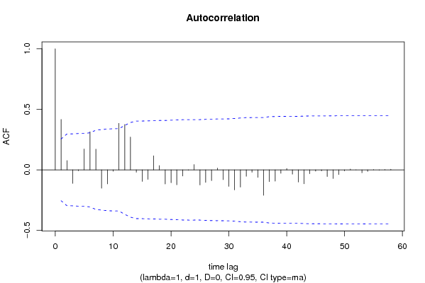
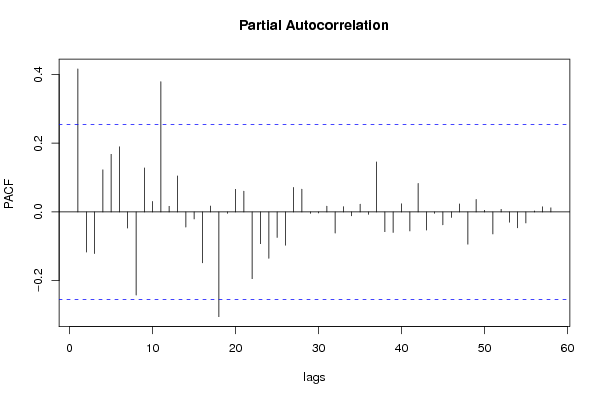
Title produced by software

(Partial) Autocorrelation Function

Date of computation

Sat, 21 Nov 2009 04:01:08 -0700

Cite this page as follows

Statistical Computations at FreeStatistics.org, Office for Research Development and Education, URL https://freestatistics.org/blog/index.php?v=date/2009/Nov/21/t1258801312k3ykqfbk1ps7anr.htm/, Retrieved Sun, 28 Apr 2024 11:04:51 +0000

Statistical Computations at FreeStatistics.org, Office for Research Development and Education, URL https://freestatistics.org/blog/index.php?pk=58528, Retrieved Sun, 28 Apr 2024 11:04:51 +0000

QR Codes:

Paste this QR Code to cite your computation.

Original text written by user:

IsPrivate?

No (this computation is public)

User-defined keywords

Estimated Impact

237

Family? (F = Feedback message, R = changed R code, M = changed R Module, P = changed Parameters, D = changed Data)

-     [Kendall tau Correlation Matrix] [Correlatie tussen...] [2007-11-03 21:44:17] [0b2d8ed757c467aee7199cdee05779c9]
- RMPD  [(Partial) Autocorrelation Function] [WS 8 01] [2009-11-21 08:59:55] [6e4e01d7eb22a9f33d58ebb35753a195]
-   PD      [(Partial) Autocorrelation Function] [WS 8 02] [2009-11-21 11:01:08] [2e4ef2c1b76db9b31c0a03b96e94ad77] [Current]
-   P         [(Partial) Autocorrelation Function] [WS 8 03] [2009-11-21 11:02:54] [6e4e01d7eb22a9f33d58ebb35753a195] 
-   P           [(Partial) Autocorrelation Function] [WS 8 04] [2009-11-21 11:06:04] [6e4e01d7eb22a9f33d58ebb35753a195] 
-   P             [(Partial) Autocorrelation Function] [ws 8 01b] [2009-11-24 22:56:18] [6e4e01d7eb22a9f33d58ebb35753a195] 
-   P           [(Partial) Autocorrelation Function] [ws9] [2009-11-29 12:25:47] [6e4e01d7eb22a9f33d58ebb35753a195] 
- RMPD            [Harrell-Davis Quantiles] [WS 9 H] [2009-12-01 21:25:24] [6e4e01d7eb22a9f33d58ebb35753a195] 
-    D              [Harrell-Davis Quantiles] [significantie res...] [2009-12-29 16:01:07] [b5ba85a7ae9f50cb97d92cbc56161b32] 
- RMPD            [Mean Plot] [ws 9 m] [2009-12-01 21:28:00] [6e4e01d7eb22a9f33d58ebb35753a195] 

Feedback Forum

Post a new message

Dataseries X:

Download CSV

Histogram

Boxplots

Summary of computational transaction
Raw Input	view raw input (R code)
Raw Output	view raw output of R engine
Computing time	1 seconds
R Server	'Gwilym Jenkins' @ 72.249.127.135

\begin{tabular}{lllllllll}
\hline
Summary of computational transaction \tabularnewline
Raw Input & view raw input (R code)  \tabularnewline
Raw Output & view raw output of R engine  \tabularnewline
Computing time & 1 seconds \tabularnewline
R Server & 'Gwilym Jenkins' @ 72.249.127.135 \tabularnewline
\hline
\end{tabular}
%Source: https://freestatistics.org/blog/index.php?pk=58528&T=0

[TABLE]
[ROW][C]Summary of computational transaction[/C][/ROW]
[ROW][C]Raw Input[/C][C]view raw input (R code) [/C][/ROW]
[ROW][C]Raw Output[/C][C]view raw output of R engine [/C][/ROW]
[ROW][C]Computing time[/C][C]1 seconds[/C][/ROW]
[ROW][C]R Server[/C][C]'Gwilym Jenkins' @ 72.249.127.135[/C][/ROW]
[/TABLE]
Source: https://freestatistics.org/blog/index.php?pk=58528&T=0

Globally Unique Identifier (entire table): ba.freestatistics.org/blog/index.php?pk=58528&T=0

As an alternative you can also use a QR Code:

The GUIDs for individual cells are displayed in the table below:

Summary of computational transaction
Raw Input	view raw input (R code)
Raw Output	view raw output of R engine
Computing time	1 seconds
R Server	'Gwilym Jenkins' @ 72.249.127.135

Autocorrelation Function
Time lag k	ACF(k)	T-STAT	P-value
1	0.41632	3.1978	0.001114
2	0.076697	0.5891	0.279014
3	-0.112083	-0.8609	0.196383
4	-0.00739	-0.0568	0.477462
5	0.172541	1.3253	0.095089
6	0.314849	2.4184	0.009347
7	0.170664	1.3109	0.097486
8	-0.151973	-1.1673	0.123888
9	-0.11594	-0.8906	0.188394
10	-0.011391	-0.0875	0.465286
11	0.38421	2.9512	0.002268
12	0.374897	2.8796	0.00277
13	0.271303	2.0839	0.020754
14	-0.019703	-0.1513	0.44011
15	-0.095952	-0.737	0.232016
16	-0.078996	-0.6068	0.273164
17	0.115967	0.8908	0.188338
18	0.034786	0.2672	0.395126
19	-0.11715	-0.8998	0.185931
20	-0.106703	-0.8196	0.20787
21	-0.123287	-0.947	0.173754
22	-0.051185	-0.3932	0.34781
23	-0.001978	-0.0152	0.493965
24	0.043653	0.3353	0.369291
25	-0.124832	-0.9589	0.170772
26	-0.103557	-0.7954	0.214774
27	-0.088949	-0.6832	0.248567
28	0.014742	0.1132	0.455113
29	-0.081337	-0.6248	0.267268
30	-0.136832	-1.051	0.148766
31	-0.165966	-1.2748	0.103688
32	-0.142771	-1.0966	0.138627
33	-0.053127	-0.4081	0.342347
34	-0.019919	-0.153	0.43946
35	-0.061795	-0.4747	0.318393
36	-0.210326	-1.6155	0.055764
37	-0.097409	-0.7482	0.228651
38	-0.093264	-0.7164	0.238293
39	-0.028542	-0.2192	0.413612
40	0.011029	0.0847	0.466388
41	-0.035533	-0.2729	0.392928
42	-0.100939	-0.7753	0.220622
43	-0.115105	-0.8841	0.190104
44	-0.032215	-0.2474	0.40271
45	-0.01118	-0.0859	0.465929
46	-0.008717	-0.067	0.47342
47	-0.05568	-0.4277	0.335218
48	-0.071667	-0.5505	0.292032
49	-0.038504	-0.2958	0.384229
50	-0.008991	-0.0691	0.472588
51	0.006412	0.0493	0.480442
52	0.000908	0.007	0.497229
53	-0.023745	-0.1824	0.427951
54	-0.013104	-0.1007	0.460084
55	0.002395	0.0184	0.492691
56	-0.001926	-0.0148	0.494122
57	0.003052	0.0234	0.490687
58	0.005237	0.0402	0.484024
59	NA	NA	NA
60	NA	NA	NA

\begin{tabular}{lllllllll}
\hline
Autocorrelation Function \tabularnewline
Time lag k & ACF(k) & T-STAT & P-value \tabularnewline
1 & 0.41632 & 3.1978 & 0.001114 \tabularnewline
2 & 0.076697 & 0.5891 & 0.279014 \tabularnewline
3 & -0.112083 & -0.8609 & 0.196383 \tabularnewline
4 & -0.00739 & -0.0568 & 0.477462 \tabularnewline
5 & 0.172541 & 1.3253 & 0.095089 \tabularnewline
6 & 0.314849 & 2.4184 & 0.009347 \tabularnewline
7 & 0.170664 & 1.3109 & 0.097486 \tabularnewline
8 & -0.151973 & -1.1673 & 0.123888 \tabularnewline
9 & -0.11594 & -0.8906 & 0.188394 \tabularnewline
10 & -0.011391 & -0.0875 & 0.465286 \tabularnewline
11 & 0.38421 & 2.9512 & 0.002268 \tabularnewline
12 & 0.374897 & 2.8796 & 0.00277 \tabularnewline
13 & 0.271303 & 2.0839 & 0.020754 \tabularnewline
14 & -0.019703 & -0.1513 & 0.44011 \tabularnewline
15 & -0.095952 & -0.737 & 0.232016 \tabularnewline
16 & -0.078996 & -0.6068 & 0.273164 \tabularnewline
17 & 0.115967 & 0.8908 & 0.188338 \tabularnewline
18 & 0.034786 & 0.2672 & 0.395126 \tabularnewline
19 & -0.11715 & -0.8998 & 0.185931 \tabularnewline
20 & -0.106703 & -0.8196 & 0.20787 \tabularnewline
21 & -0.123287 & -0.947 & 0.173754 \tabularnewline
22 & -0.051185 & -0.3932 & 0.34781 \tabularnewline
23 & -0.001978 & -0.0152 & 0.493965 \tabularnewline
24 & 0.043653 & 0.3353 & 0.369291 \tabularnewline
25 & -0.124832 & -0.9589 & 0.170772 \tabularnewline
26 & -0.103557 & -0.7954 & 0.214774 \tabularnewline
27 & -0.088949 & -0.6832 & 0.248567 \tabularnewline
28 & 0.014742 & 0.1132 & 0.455113 \tabularnewline
29 & -0.081337 & -0.6248 & 0.267268 \tabularnewline
30 & -0.136832 & -1.051 & 0.148766 \tabularnewline
31 & -0.165966 & -1.2748 & 0.103688 \tabularnewline
32 & -0.142771 & -1.0966 & 0.138627 \tabularnewline
33 & -0.053127 & -0.4081 & 0.342347 \tabularnewline
34 & -0.019919 & -0.153 & 0.43946 \tabularnewline
35 & -0.061795 & -0.4747 & 0.318393 \tabularnewline
36 & -0.210326 & -1.6155 & 0.055764 \tabularnewline
37 & -0.097409 & -0.7482 & 0.228651 \tabularnewline
38 & -0.093264 & -0.7164 & 0.238293 \tabularnewline
39 & -0.028542 & -0.2192 & 0.413612 \tabularnewline
40 & 0.011029 & 0.0847 & 0.466388 \tabularnewline
41 & -0.035533 & -0.2729 & 0.392928 \tabularnewline
42 & -0.100939 & -0.7753 & 0.220622 \tabularnewline
43 & -0.115105 & -0.8841 & 0.190104 \tabularnewline
44 & -0.032215 & -0.2474 & 0.40271 \tabularnewline
45 & -0.01118 & -0.0859 & 0.465929 \tabularnewline
46 & -0.008717 & -0.067 & 0.47342 \tabularnewline
47 & -0.05568 & -0.4277 & 0.335218 \tabularnewline
48 & -0.071667 & -0.5505 & 0.292032 \tabularnewline
49 & -0.038504 & -0.2958 & 0.384229 \tabularnewline
50 & -0.008991 & -0.0691 & 0.472588 \tabularnewline
51 & 0.006412 & 0.0493 & 0.480442 \tabularnewline
52 & 0.000908 & 0.007 & 0.497229 \tabularnewline
53 & -0.023745 & -0.1824 & 0.427951 \tabularnewline
54 & -0.013104 & -0.1007 & 0.460084 \tabularnewline
55 & 0.002395 & 0.0184 & 0.492691 \tabularnewline
56 & -0.001926 & -0.0148 & 0.494122 \tabularnewline
57 & 0.003052 & 0.0234 & 0.490687 \tabularnewline
58 & 0.005237 & 0.0402 & 0.484024 \tabularnewline
59 & NA & NA & NA \tabularnewline
60 & NA & NA & NA \tabularnewline
\hline
\end{tabular}
%Source: https://freestatistics.org/blog/index.php?pk=58528&T=1

[TABLE]
[ROW][C]Autocorrelation Function[/C][/ROW]
[ROW][C]Time lag k[/C][C]ACF(k)[/C][C]T-STAT[/C][C]P-value[/C][/ROW]
[ROW][C]1[/C][C]0.41632[/C][C]3.1978[/C][C]0.001114[/C][/ROW]
[ROW][C]2[/C][C]0.076697[/C][C]0.5891[/C][C]0.279014[/C][/ROW]
[ROW][C]3[/C][C]-0.112083[/C][C]-0.8609[/C][C]0.196383[/C][/ROW]
[ROW][C]4[/C][C]-0.00739[/C][C]-0.0568[/C][C]0.477462[/C][/ROW]
[ROW][C]5[/C][C]0.172541[/C][C]1.3253[/C][C]0.095089[/C][/ROW]
[ROW][C]6[/C][C]0.314849[/C][C]2.4184[/C][C]0.009347[/C][/ROW]
[ROW][C]7[/C][C]0.170664[/C][C]1.3109[/C][C]0.097486[/C][/ROW]
[ROW][C]8[/C][C]-0.151973[/C][C]-1.1673[/C][C]0.123888[/C][/ROW]
[ROW][C]9[/C][C]-0.11594[/C][C]-0.8906[/C][C]0.188394[/C][/ROW]
[ROW][C]10[/C][C]-0.011391[/C][C]-0.0875[/C][C]0.465286[/C][/ROW]
[ROW][C]11[/C][C]0.38421[/C][C]2.9512[/C][C]0.002268[/C][/ROW]
[ROW][C]12[/C][C]0.374897[/C][C]2.8796[/C][C]0.00277[/C][/ROW]
[ROW][C]13[/C][C]0.271303[/C][C]2.0839[/C][C]0.020754[/C][/ROW]
[ROW][C]14[/C][C]-0.019703[/C][C]-0.1513[/C][C]0.44011[/C][/ROW]
[ROW][C]15[/C][C]-0.095952[/C][C]-0.737[/C][C]0.232016[/C][/ROW]
[ROW][C]16[/C][C]-0.078996[/C][C]-0.6068[/C][C]0.273164[/C][/ROW]
[ROW][C]17[/C][C]0.115967[/C][C]0.8908[/C][C]0.188338[/C][/ROW]
[ROW][C]18[/C][C]0.034786[/C][C]0.2672[/C][C]0.395126[/C][/ROW]
[ROW][C]19[/C][C]-0.11715[/C][C]-0.8998[/C][C]0.185931[/C][/ROW]
[ROW][C]20[/C][C]-0.106703[/C][C]-0.8196[/C][C]0.20787[/C][/ROW]
[ROW][C]21[/C][C]-0.123287[/C][C]-0.947[/C][C]0.173754[/C][/ROW]
[ROW][C]22[/C][C]-0.051185[/C][C]-0.3932[/C][C]0.34781[/C][/ROW]
[ROW][C]23[/C][C]-0.001978[/C][C]-0.0152[/C][C]0.493965[/C][/ROW]
[ROW][C]24[/C][C]0.043653[/C][C]0.3353[/C][C]0.369291[/C][/ROW]
[ROW][C]25[/C][C]-0.124832[/C][C]-0.9589[/C][C]0.170772[/C][/ROW]
[ROW][C]26[/C][C]-0.103557[/C][C]-0.7954[/C][C]0.214774[/C][/ROW]
[ROW][C]27[/C][C]-0.088949[/C][C]-0.6832[/C][C]0.248567[/C][/ROW]
[ROW][C]28[/C][C]0.014742[/C][C]0.1132[/C][C]0.455113[/C][/ROW]
[ROW][C]29[/C][C]-0.081337[/C][C]-0.6248[/C][C]0.267268[/C][/ROW]
[ROW][C]30[/C][C]-0.136832[/C][C]-1.051[/C][C]0.148766[/C][/ROW]
[ROW][C]31[/C][C]-0.165966[/C][C]-1.2748[/C][C]0.103688[/C][/ROW]
[ROW][C]32[/C][C]-0.142771[/C][C]-1.0966[/C][C]0.138627[/C][/ROW]
[ROW][C]33[/C][C]-0.053127[/C][C]-0.4081[/C][C]0.342347[/C][/ROW]
[ROW][C]34[/C][C]-0.019919[/C][C]-0.153[/C][C]0.43946[/C][/ROW]
[ROW][C]35[/C][C]-0.061795[/C][C]-0.4747[/C][C]0.318393[/C][/ROW]
[ROW][C]36[/C][C]-0.210326[/C][C]-1.6155[/C][C]0.055764[/C][/ROW]
[ROW][C]37[/C][C]-0.097409[/C][C]-0.7482[/C][C]0.228651[/C][/ROW]
[ROW][C]38[/C][C]-0.093264[/C][C]-0.7164[/C][C]0.238293[/C][/ROW]
[ROW][C]39[/C][C]-0.028542[/C][C]-0.2192[/C][C]0.413612[/C][/ROW]
[ROW][C]40[/C][C]0.011029[/C][C]0.0847[/C][C]0.466388[/C][/ROW]
[ROW][C]41[/C][C]-0.035533[/C][C]-0.2729[/C][C]0.392928[/C][/ROW]
[ROW][C]42[/C][C]-0.100939[/C][C]-0.7753[/C][C]0.220622[/C][/ROW]
[ROW][C]43[/C][C]-0.115105[/C][C]-0.8841[/C][C]0.190104[/C][/ROW]
[ROW][C]44[/C][C]-0.032215[/C][C]-0.2474[/C][C]0.40271[/C][/ROW]
[ROW][C]45[/C][C]-0.01118[/C][C]-0.0859[/C][C]0.465929[/C][/ROW]
[ROW][C]46[/C][C]-0.008717[/C][C]-0.067[/C][C]0.47342[/C][/ROW]
[ROW][C]47[/C][C]-0.05568[/C][C]-0.4277[/C][C]0.335218[/C][/ROW]
[ROW][C]48[/C][C]-0.071667[/C][C]-0.5505[/C][C]0.292032[/C][/ROW]
[ROW][C]49[/C][C]-0.038504[/C][C]-0.2958[/C][C]0.384229[/C][/ROW]
[ROW][C]50[/C][C]-0.008991[/C][C]-0.0691[/C][C]0.472588[/C][/ROW]
[ROW][C]51[/C][C]0.006412[/C][C]0.0493[/C][C]0.480442[/C][/ROW]
[ROW][C]52[/C][C]0.000908[/C][C]0.007[/C][C]0.497229[/C][/ROW]
[ROW][C]53[/C][C]-0.023745[/C][C]-0.1824[/C][C]0.427951[/C][/ROW]
[ROW][C]54[/C][C]-0.013104[/C][C]-0.1007[/C][C]0.460084[/C][/ROW]
[ROW][C]55[/C][C]0.002395[/C][C]0.0184[/C][C]0.492691[/C][/ROW]
[ROW][C]56[/C][C]-0.001926[/C][C]-0.0148[/C][C]0.494122[/C][/ROW]
[ROW][C]57[/C][C]0.003052[/C][C]0.0234[/C][C]0.490687[/C][/ROW]
[ROW][C]58[/C][C]0.005237[/C][C]0.0402[/C][C]0.484024[/C][/ROW]
[ROW][C]59[/C][C]NA[/C][C]NA[/C][C]NA[/C][/ROW]
[ROW][C]60[/C][C]NA[/C][C]NA[/C][C]NA[/C][/ROW]
[/TABLE]
Source: https://freestatistics.org/blog/index.php?pk=58528&T=1

Globally Unique Identifier (entire table): ba.freestatistics.org/blog/index.php?pk=58528&T=1

As an alternative you can also use a QR Code:

The GUIDs for individual cells are displayed in the table below:

Autocorrelation Function
Time lag k	ACF(k)	T-STAT	P-value
1	0.41632	3.1978	0.001114
2	0.076697	0.5891	0.279014
3	-0.112083	-0.8609	0.196383
4	-0.00739	-0.0568	0.477462
5	0.172541	1.3253	0.095089
6	0.314849	2.4184	0.009347
7	0.170664	1.3109	0.097486
8	-0.151973	-1.1673	0.123888
9	-0.11594	-0.8906	0.188394
10	-0.011391	-0.0875	0.465286
11	0.38421	2.9512	0.002268
12	0.374897	2.8796	0.00277
13	0.271303	2.0839	0.020754
14	-0.019703	-0.1513	0.44011
15	-0.095952	-0.737	0.232016
16	-0.078996	-0.6068	0.273164
17	0.115967	0.8908	0.188338
18	0.034786	0.2672	0.395126
19	-0.11715	-0.8998	0.185931
20	-0.106703	-0.8196	0.20787
21	-0.123287	-0.947	0.173754
22	-0.051185	-0.3932	0.34781
23	-0.001978	-0.0152	0.493965
24	0.043653	0.3353	0.369291
25	-0.124832	-0.9589	0.170772
26	-0.103557	-0.7954	0.214774
27	-0.088949	-0.6832	0.248567
28	0.014742	0.1132	0.455113
29	-0.081337	-0.6248	0.267268
30	-0.136832	-1.051	0.148766
31	-0.165966	-1.2748	0.103688
32	-0.142771	-1.0966	0.138627
33	-0.053127	-0.4081	0.342347
34	-0.019919	-0.153	0.43946
35	-0.061795	-0.4747	0.318393
36	-0.210326	-1.6155	0.055764
37	-0.097409	-0.7482	0.228651
38	-0.093264	-0.7164	0.238293
39	-0.028542	-0.2192	0.413612
40	0.011029	0.0847	0.466388
41	-0.035533	-0.2729	0.392928
42	-0.100939	-0.7753	0.220622
43	-0.115105	-0.8841	0.190104
44	-0.032215	-0.2474	0.40271
45	-0.01118	-0.0859	0.465929
46	-0.008717	-0.067	0.47342
47	-0.05568	-0.4277	0.335218
48	-0.071667	-0.5505	0.292032
49	-0.038504	-0.2958	0.384229
50	-0.008991	-0.0691	0.472588
51	0.006412	0.0493	0.480442
52	0.000908	0.007	0.497229
53	-0.023745	-0.1824	0.427951
54	-0.013104	-0.1007	0.460084
55	0.002395	0.0184	0.492691
56	-0.001926	-0.0148	0.494122
57	0.003052	0.0234	0.490687
58	0.005237	0.0402	0.484024
59	NA	NA	NA
60	NA	NA	NA

Partial Autocorrelation Function
Time lag k	PACF(k)	T-STAT	P-value
1	0.41632	3.1978	0.001114
2	-0.116884	-0.8978	0.186471
3	-0.121519	-0.9334	0.177208
4	0.122433	0.9404	0.175417
5	0.167603	1.2874	0.101494
6	0.189684	1.457	0.075211
7	-0.047036	-0.3613	0.359587
8	-0.242216	-1.8605	0.0339
9	0.12786	0.9821	0.165027
10	0.030622	0.2352	0.40743
11	0.379101	2.9119	0.002532
12	0.016369	0.1257	0.450185
13	0.104565	0.8032	0.212548
14	-0.044164	-0.3392	0.36782
15	-0.020599	-0.1582	0.43741
16	-0.148269	-1.1389	0.129679
17	0.016911	0.1299	0.448546
18	-0.30509	-2.3434	0.011248
19	-0.004059	-0.0312	0.487618
20	0.065685	0.5045	0.307882
21	0.060226	0.4626	0.322674
22	-0.194641	-1.4951	0.070114
23	-0.092736	-0.7123	0.239537
24	-0.135252	-1.0389	0.151547
25	-0.074269	-0.5705	0.285261
26	-0.096898	-0.7443	0.229829
27	0.071259	0.5473	0.293102
28	0.066254	0.5089	0.306358
29	-0.004293	-0.033	0.486902
30	-0.003117	-0.0239	0.49049
31	0.016705	0.1283	0.44917
32	-0.061761	-0.4744	0.318484
33	0.015071	0.1158	0.454116
34	-0.011424	-0.0878	0.465185
35	0.022594	0.1735	0.431407
36	-0.006888	-0.0529	0.478992
37	0.145556	1.118	0.134042
38	-0.057775	-0.4438	0.329414
39	-0.059697	-0.4585	0.324123
40	0.023437	0.18	0.428875
41	-0.0556	-0.4271	0.335441
42	0.083019	0.6377	0.263075
43	-0.052757	-0.4052	0.343386
44	-0.004185	-0.0321	0.487232
45	-0.037471	-0.2878	0.387247
46	-0.016179	-0.1243	0.45076
47	0.02317	0.178	0.429677
48	-0.094055	-0.7224	0.236437
49	0.036326	0.279	0.390599
50	0.004745	0.0364	0.485524
51	-0.064161	-0.4928	0.31198
52	0.007385	0.0567	0.477478
53	-0.029828	-0.2291	0.409787
54	-0.046247	-0.3552	0.361841
55	-0.032083	-0.2464	0.403101
56	0.002947	0.0226	0.491009
57	0.014735	0.1132	0.455134
58	0.011971	0.0919	0.463525
59	NA	NA	NA
60	NA	NA	NA

\begin{tabular}{lllllllll}
\hline
Partial Autocorrelation Function \tabularnewline
Time lag k & PACF(k) & T-STAT & P-value \tabularnewline
1 & 0.41632 & 3.1978 & 0.001114 \tabularnewline
2 & -0.116884 & -0.8978 & 0.186471 \tabularnewline
3 & -0.121519 & -0.9334 & 0.177208 \tabularnewline
4 & 0.122433 & 0.9404 & 0.175417 \tabularnewline
5 & 0.167603 & 1.2874 & 0.101494 \tabularnewline
6 & 0.189684 & 1.457 & 0.075211 \tabularnewline
7 & -0.047036 & -0.3613 & 0.359587 \tabularnewline
8 & -0.242216 & -1.8605 & 0.0339 \tabularnewline
9 & 0.12786 & 0.9821 & 0.165027 \tabularnewline
10 & 0.030622 & 0.2352 & 0.40743 \tabularnewline
11 & 0.379101 & 2.9119 & 0.002532 \tabularnewline
12 & 0.016369 & 0.1257 & 0.450185 \tabularnewline
13 & 0.104565 & 0.8032 & 0.212548 \tabularnewline
14 & -0.044164 & -0.3392 & 0.36782 \tabularnewline
15 & -0.020599 & -0.1582 & 0.43741 \tabularnewline
16 & -0.148269 & -1.1389 & 0.129679 \tabularnewline
17 & 0.016911 & 0.1299 & 0.448546 \tabularnewline
18 & -0.30509 & -2.3434 & 0.011248 \tabularnewline
19 & -0.004059 & -0.0312 & 0.487618 \tabularnewline
20 & 0.065685 & 0.5045 & 0.307882 \tabularnewline
21 & 0.060226 & 0.4626 & 0.322674 \tabularnewline
22 & -0.194641 & -1.4951 & 0.070114 \tabularnewline
23 & -0.092736 & -0.7123 & 0.239537 \tabularnewline
24 & -0.135252 & -1.0389 & 0.151547 \tabularnewline
25 & -0.074269 & -0.5705 & 0.285261 \tabularnewline
26 & -0.096898 & -0.7443 & 0.229829 \tabularnewline
27 & 0.071259 & 0.5473 & 0.293102 \tabularnewline
28 & 0.066254 & 0.5089 & 0.306358 \tabularnewline
29 & -0.004293 & -0.033 & 0.486902 \tabularnewline
30 & -0.003117 & -0.0239 & 0.49049 \tabularnewline
31 & 0.016705 & 0.1283 & 0.44917 \tabularnewline
32 & -0.061761 & -0.4744 & 0.318484 \tabularnewline
33 & 0.015071 & 0.1158 & 0.454116 \tabularnewline
34 & -0.011424 & -0.0878 & 0.465185 \tabularnewline
35 & 0.022594 & 0.1735 & 0.431407 \tabularnewline
36 & -0.006888 & -0.0529 & 0.478992 \tabularnewline
37 & 0.145556 & 1.118 & 0.134042 \tabularnewline
38 & -0.057775 & -0.4438 & 0.329414 \tabularnewline
39 & -0.059697 & -0.4585 & 0.324123 \tabularnewline
40 & 0.023437 & 0.18 & 0.428875 \tabularnewline
41 & -0.0556 & -0.4271 & 0.335441 \tabularnewline
42 & 0.083019 & 0.6377 & 0.263075 \tabularnewline
43 & -0.052757 & -0.4052 & 0.343386 \tabularnewline
44 & -0.004185 & -0.0321 & 0.487232 \tabularnewline
45 & -0.037471 & -0.2878 & 0.387247 \tabularnewline
46 & -0.016179 & -0.1243 & 0.45076 \tabularnewline
47 & 0.02317 & 0.178 & 0.429677 \tabularnewline
48 & -0.094055 & -0.7224 & 0.236437 \tabularnewline
49 & 0.036326 & 0.279 & 0.390599 \tabularnewline
50 & 0.004745 & 0.0364 & 0.485524 \tabularnewline
51 & -0.064161 & -0.4928 & 0.31198 \tabularnewline
52 & 0.007385 & 0.0567 & 0.477478 \tabularnewline
53 & -0.029828 & -0.2291 & 0.409787 \tabularnewline
54 & -0.046247 & -0.3552 & 0.361841 \tabularnewline
55 & -0.032083 & -0.2464 & 0.403101 \tabularnewline
56 & 0.002947 & 0.0226 & 0.491009 \tabularnewline
57 & 0.014735 & 0.1132 & 0.455134 \tabularnewline
58 & 0.011971 & 0.0919 & 0.463525 \tabularnewline
59 & NA & NA & NA \tabularnewline
60 & NA & NA & NA \tabularnewline
\hline
\end{tabular}
%Source: https://freestatistics.org/blog/index.php?pk=58528&T=2

[TABLE]
[ROW][C]Partial Autocorrelation Function[/C][/ROW]
[ROW][C]Time lag k[/C][C]PACF(k)[/C][C]T-STAT[/C][C]P-value[/C][/ROW]
[ROW][C]1[/C][C]0.41632[/C][C]3.1978[/C][C]0.001114[/C][/ROW]
[ROW][C]2[/C][C]-0.116884[/C][C]-0.8978[/C][C]0.186471[/C][/ROW]
[ROW][C]3[/C][C]-0.121519[/C][C]-0.9334[/C][C]0.177208[/C][/ROW]
[ROW][C]4[/C][C]0.122433[/C][C]0.9404[/C][C]0.175417[/C][/ROW]
[ROW][C]5[/C][C]0.167603[/C][C]1.2874[/C][C]0.101494[/C][/ROW]
[ROW][C]6[/C][C]0.189684[/C][C]1.457[/C][C]0.075211[/C][/ROW]
[ROW][C]7[/C][C]-0.047036[/C][C]-0.3613[/C][C]0.359587[/C][/ROW]
[ROW][C]8[/C][C]-0.242216[/C][C]-1.8605[/C][C]0.0339[/C][/ROW]
[ROW][C]9[/C][C]0.12786[/C][C]0.9821[/C][C]0.165027[/C][/ROW]
[ROW][C]10[/C][C]0.030622[/C][C]0.2352[/C][C]0.40743[/C][/ROW]
[ROW][C]11[/C][C]0.379101[/C][C]2.9119[/C][C]0.002532[/C][/ROW]
[ROW][C]12[/C][C]0.016369[/C][C]0.1257[/C][C]0.450185[/C][/ROW]
[ROW][C]13[/C][C]0.104565[/C][C]0.8032[/C][C]0.212548[/C][/ROW]
[ROW][C]14[/C][C]-0.044164[/C][C]-0.3392[/C][C]0.36782[/C][/ROW]
[ROW][C]15[/C][C]-0.020599[/C][C]-0.1582[/C][C]0.43741[/C][/ROW]
[ROW][C]16[/C][C]-0.148269[/C][C]-1.1389[/C][C]0.129679[/C][/ROW]
[ROW][C]17[/C][C]0.016911[/C][C]0.1299[/C][C]0.448546[/C][/ROW]
[ROW][C]18[/C][C]-0.30509[/C][C]-2.3434[/C][C]0.011248[/C][/ROW]
[ROW][C]19[/C][C]-0.004059[/C][C]-0.0312[/C][C]0.487618[/C][/ROW]
[ROW][C]20[/C][C]0.065685[/C][C]0.5045[/C][C]0.307882[/C][/ROW]
[ROW][C]21[/C][C]0.060226[/C][C]0.4626[/C][C]0.322674[/C][/ROW]
[ROW][C]22[/C][C]-0.194641[/C][C]-1.4951[/C][C]0.070114[/C][/ROW]
[ROW][C]23[/C][C]-0.092736[/C][C]-0.7123[/C][C]0.239537[/C][/ROW]
[ROW][C]24[/C][C]-0.135252[/C][C]-1.0389[/C][C]0.151547[/C][/ROW]
[ROW][C]25[/C][C]-0.074269[/C][C]-0.5705[/C][C]0.285261[/C][/ROW]
[ROW][C]26[/C][C]-0.096898[/C][C]-0.7443[/C][C]0.229829[/C][/ROW]
[ROW][C]27[/C][C]0.071259[/C][C]0.5473[/C][C]0.293102[/C][/ROW]
[ROW][C]28[/C][C]0.066254[/C][C]0.5089[/C][C]0.306358[/C][/ROW]
[ROW][C]29[/C][C]-0.004293[/C][C]-0.033[/C][C]0.486902[/C][/ROW]
[ROW][C]30[/C][C]-0.003117[/C][C]-0.0239[/C][C]0.49049[/C][/ROW]
[ROW][C]31[/C][C]0.016705[/C][C]0.1283[/C][C]0.44917[/C][/ROW]
[ROW][C]32[/C][C]-0.061761[/C][C]-0.4744[/C][C]0.318484[/C][/ROW]
[ROW][C]33[/C][C]0.015071[/C][C]0.1158[/C][C]0.454116[/C][/ROW]
[ROW][C]34[/C][C]-0.011424[/C][C]-0.0878[/C][C]0.465185[/C][/ROW]
[ROW][C]35[/C][C]0.022594[/C][C]0.1735[/C][C]0.431407[/C][/ROW]
[ROW][C]36[/C][C]-0.006888[/C][C]-0.0529[/C][C]0.478992[/C][/ROW]
[ROW][C]37[/C][C]0.145556[/C][C]1.118[/C][C]0.134042[/C][/ROW]
[ROW][C]38[/C][C]-0.057775[/C][C]-0.4438[/C][C]0.329414[/C][/ROW]
[ROW][C]39[/C][C]-0.059697[/C][C]-0.4585[/C][C]0.324123[/C][/ROW]
[ROW][C]40[/C][C]0.023437[/C][C]0.18[/C][C]0.428875[/C][/ROW]
[ROW][C]41[/C][C]-0.0556[/C][C]-0.4271[/C][C]0.335441[/C][/ROW]
[ROW][C]42[/C][C]0.083019[/C][C]0.6377[/C][C]0.263075[/C][/ROW]
[ROW][C]43[/C][C]-0.052757[/C][C]-0.4052[/C][C]0.343386[/C][/ROW]
[ROW][C]44[/C][C]-0.004185[/C][C]-0.0321[/C][C]0.487232[/C][/ROW]
[ROW][C]45[/C][C]-0.037471[/C][C]-0.2878[/C][C]0.387247[/C][/ROW]
[ROW][C]46[/C][C]-0.016179[/C][C]-0.1243[/C][C]0.45076[/C][/ROW]
[ROW][C]47[/C][C]0.02317[/C][C]0.178[/C][C]0.429677[/C][/ROW]
[ROW][C]48[/C][C]-0.094055[/C][C]-0.7224[/C][C]0.236437[/C][/ROW]
[ROW][C]49[/C][C]0.036326[/C][C]0.279[/C][C]0.390599[/C][/ROW]
[ROW][C]50[/C][C]0.004745[/C][C]0.0364[/C][C]0.485524[/C][/ROW]
[ROW][C]51[/C][C]-0.064161[/C][C]-0.4928[/C][C]0.31198[/C][/ROW]
[ROW][C]52[/C][C]0.007385[/C][C]0.0567[/C][C]0.477478[/C][/ROW]
[ROW][C]53[/C][C]-0.029828[/C][C]-0.2291[/C][C]0.409787[/C][/ROW]
[ROW][C]54[/C][C]-0.046247[/C][C]-0.3552[/C][C]0.361841[/C][/ROW]
[ROW][C]55[/C][C]-0.032083[/C][C]-0.2464[/C][C]0.403101[/C][/ROW]
[ROW][C]56[/C][C]0.002947[/C][C]0.0226[/C][C]0.491009[/C][/ROW]
[ROW][C]57[/C][C]0.014735[/C][C]0.1132[/C][C]0.455134[/C][/ROW]
[ROW][C]58[/C][C]0.011971[/C][C]0.0919[/C][C]0.463525[/C][/ROW]
[ROW][C]59[/C][C]NA[/C][C]NA[/C][C]NA[/C][/ROW]
[ROW][C]60[/C][C]NA[/C][C]NA[/C][C]NA[/C][/ROW]
[/TABLE]
Source: https://freestatistics.org/blog/index.php?pk=58528&T=2

Globally Unique Identifier (entire table): ba.freestatistics.org/blog/index.php?pk=58528&T=2

As an alternative you can also use a QR Code:

The GUIDs for individual cells are displayed in the table below:

Partial Autocorrelation Function
Time lag k	PACF(k)	T-STAT	P-value
1	0.41632	3.1978	0.001114
2	-0.116884	-0.8978	0.186471
3	-0.121519	-0.9334	0.177208
4	0.122433	0.9404	0.175417
5	0.167603	1.2874	0.101494
6	0.189684	1.457	0.075211
7	-0.047036	-0.3613	0.359587
8	-0.242216	-1.8605	0.0339
9	0.12786	0.9821	0.165027
10	0.030622	0.2352	0.40743
11	0.379101	2.9119	0.002532
12	0.016369	0.1257	0.450185
13	0.104565	0.8032	0.212548
14	-0.044164	-0.3392	0.36782
15	-0.020599	-0.1582	0.43741
16	-0.148269	-1.1389	0.129679
17	0.016911	0.1299	0.448546
18	-0.30509	-2.3434	0.011248
19	-0.004059	-0.0312	0.487618
20	0.065685	0.5045	0.307882
21	0.060226	0.4626	0.322674
22	-0.194641	-1.4951	0.070114
23	-0.092736	-0.7123	0.239537
24	-0.135252	-1.0389	0.151547
25	-0.074269	-0.5705	0.285261
26	-0.096898	-0.7443	0.229829
27	0.071259	0.5473	0.293102
28	0.066254	0.5089	0.306358
29	-0.004293	-0.033	0.486902
30	-0.003117	-0.0239	0.49049
31	0.016705	0.1283	0.44917
32	-0.061761	-0.4744	0.318484
33	0.015071	0.1158	0.454116
34	-0.011424	-0.0878	0.465185
35	0.022594	0.1735	0.431407
36	-0.006888	-0.0529	0.478992
37	0.145556	1.118	0.134042
38	-0.057775	-0.4438	0.329414
39	-0.059697	-0.4585	0.324123
40	0.023437	0.18	0.428875
41	-0.0556	-0.4271	0.335441
42	0.083019	0.6377	0.263075
43	-0.052757	-0.4052	0.343386
44	-0.004185	-0.0321	0.487232
45	-0.037471	-0.2878	0.387247
46	-0.016179	-0.1243	0.45076
47	0.02317	0.178	0.429677
48	-0.094055	-0.7224	0.236437
49	0.036326	0.279	0.390599
50	0.004745	0.0364	0.485524
51	-0.064161	-0.4928	0.31198
52	0.007385	0.0567	0.477478
53	-0.029828	-0.2291	0.409787
54	-0.046247	-0.3552	0.361841
55	-0.032083	-0.2464	0.403101
56	0.002947	0.0226	0.491009
57	0.014735	0.1132	0.455134
58	0.011971	0.0919	0.463525
59	NA	NA	NA
60	NA	NA	NA

Figure 1

PNG link

Postscript link

PDF link

Figure 2

PNG link

Postscript link

PDF link

Parameters (Session):

par1 = 60 ; par2 = 1 ; par3 = 1 ; par4 = 0 ; par5 = 12 ; par6 = MA ; par7 = 0.95 ;

Parameters (R input):

par1 = 60 ; par2 = 1 ; par3 = 1 ; par4 = 0 ; par5 = 12 ; par6 = MA ; par7 = 0.95 ;

R code (references can be found in the software module):

if (par1 == 'Default') {
par1 = 10*log10(length(x))
} else {
par1 <- as.numeric(par1)
}
par2 <- as.numeric(par2)
par3 <- as.numeric(par3)
par4 <- as.numeric(par4)
par5 <- as.numeric(par5)
if (par6 == 'White Noise') par6 <- 'white' else par6 <- 'ma'
par7 <- as.numeric(par7)
if (par2 == 0) {
x <- log(x)
} else {
x <- (x ^ par2 - 1) / par2
}
if (par3 > 0) x <- diff(x,lag=1,difference=par3)
if (par4 > 0) x <- diff(x,lag=par5,difference=par4)
bitmap(file='pic1.png')
racf <- acf(x, par1, main='Autocorrelation', xlab='time lag', ylab='ACF', ci.type=par6, ci=par7, sub=paste('(lambda=',par2,', d=',par3,', D=',par4,', CI=', par7, ', CI type=',par6,')',sep=''))
dev.off()
bitmap(file='pic2.png')
rpacf <- pacf(x,par1,main='Partial Autocorrelation',xlab='lags',ylab='PACF')
dev.off()
(myacf <- c(racf$acf))
(mypacf <- c(rpacf$acf))
lengthx <- length(x)
sqrtn <- sqrt(lengthx)
load(file='createtable')
a<-table.start()
a<-table.row.start(a)
a<-table.element(a,'Autocorrelation Function',4,TRUE)
a<-table.row.end(a)
a<-table.row.start(a)
a<-table.element(a,'Time lag k',header=TRUE)
a<-table.element(a,hyperlink('basics.htm','ACF(k)','click here for more information about the Autocorrelation Function'),header=TRUE)
a<-table.element(a,'T-STAT',header=TRUE)
a<-table.element(a,'P-value',header=TRUE)
a<-table.row.end(a)
for (i in 2:(par1+1)) {
a<-table.row.start(a)
a<-table.element(a,i-1,header=TRUE)
a<-table.element(a,round(myacf[i],6))
mytstat <- myacf[i]*sqrtn
a<-table.element(a,round(mytstat,4))
a<-table.element(a,round(1-pt(abs(mytstat),lengthx),6))
a<-table.row.end(a)
}
a<-table.end(a)
table.save(a,file='mytable.tab')
a<-table.start()
a<-table.row.start(a)
a<-table.element(a,'Partial Autocorrelation Function',4,TRUE)
a<-table.row.end(a)
a<-table.row.start(a)
a<-table.element(a,'Time lag k',header=TRUE)
a<-table.element(a,hyperlink('basics.htm','PACF(k)','click here for more information about the Partial Autocorrelation Function'),header=TRUE)
a<-table.element(a,'T-STAT',header=TRUE)
a<-table.element(a,'P-value',header=TRUE)
a<-table.row.end(a)
for (i in 1:par1) {
a<-table.row.start(a)
a<-table.element(a,i,header=TRUE)
a<-table.element(a,round(mypacf[i],6))
mytstat <- mypacf[i]*sqrtn
a<-table.element(a,round(mytstat,4))
a<-table.element(a,round(1-pt(abs(mytstat),lengthx),6))
a<-table.row.end(a)
}
a<-table.end(a)
table.save(a,file='mytable1.tab')

Free Statistics

Description of Statistical Computation

Tree of Dependent Computations

Dataset

Tables (Output of Computation)

Figures (Output of Computation)

Input Parameters & R Code