Free Statistics
of Irreproducible Research!
Description of Statistical Computation | |||||||||||||||||||||||||||||||||||||||||||||||||||||||||||||||||
|---|---|---|---|---|---|---|---|---|---|---|---|---|---|---|---|---|---|---|---|---|---|---|---|---|---|---|---|---|---|---|---|---|---|---|---|---|---|---|---|---|---|---|---|---|---|---|---|---|---|---|---|---|---|---|---|---|---|---|---|---|---|---|---|---|---|
| Author's title | |||||||||||||||||||||||||||||||||||||||||||||||||||||||||||||||||
| Author | *The author of this computation has been verified* | ||||||||||||||||||||||||||||||||||||||||||||||||||||||||||||||||
| R Software Module | rwasp_edabi.wasp | ||||||||||||||||||||||||||||||||||||||||||||||||||||||||||||||||
| Title produced by software | Bivariate Explorative Data Analysis | ||||||||||||||||||||||||||||||||||||||||||||||||||||||||||||||||
| Date of computation | Wed, 25 Nov 2009 16:09:30 -0700 | ||||||||||||||||||||||||||||||||||||||||||||||||||||||||||||||||
| Cite this page as follows | Statistical Computations at FreeStatistics.org, Office for Research Development and Education, URL https://freestatistics.org/blog/index.php?v=date/2009/Nov/26/t1259190640n846mz683unsijp.htm/, Retrieved Mon, 29 Apr 2024 06:49:55 +0000 | ||||||||||||||||||||||||||||||||||||||||||||||||||||||||||||||||
| Statistical Computations at FreeStatistics.org, Office for Research Development and Education, URL https://freestatistics.org/blog/index.php?pk=59682, Retrieved Mon, 29 Apr 2024 06:49:55 +0000 | |||||||||||||||||||||||||||||||||||||||||||||||||||||||||||||||||
| QR Codes: | |||||||||||||||||||||||||||||||||||||||||||||||||||||||||||||||||
|
| |||||||||||||||||||||||||||||||||||||||||||||||||||||||||||||||||
| Original text written by user: | |||||||||||||||||||||||||||||||||||||||||||||||||||||||||||||||||
| IsPrivate? | No (this computation is public) | ||||||||||||||||||||||||||||||||||||||||||||||||||||||||||||||||
| User-defined keywords | |||||||||||||||||||||||||||||||||||||||||||||||||||||||||||||||||
| Estimated Impact | 149 | ||||||||||||||||||||||||||||||||||||||||||||||||||||||||||||||||
Tree of Dependent Computations | |||||||||||||||||||||||||||||||||||||||||||||||||||||||||||||||||
| Family? (F = Feedback message, R = changed R code, M = changed R Module, P = changed Parameters, D = changed Data) | |||||||||||||||||||||||||||||||||||||||||||||||||||||||||||||||||
| - [Bivariate Explorative Data Analysis] [SHW_WS4_Q2(1)] [2009-10-23 08:40:25] [8b1aef4e7013bd33fbc2a5833375c5f5] - M D [Bivariate Explorative Data Analysis] [Revieuw ws] [2009-11-25 23:09:30] [ac86848d66148c9c4c9404e0c9a511eb] [Current] | |||||||||||||||||||||||||||||||||||||||||||||||||||||||||||||||||
| Feedback Forum | |||||||||||||||||||||||||||||||||||||||||||||||||||||||||||||||||
Post a new message | |||||||||||||||||||||||||||||||||||||||||||||||||||||||||||||||||
Dataset | |||||||||||||||||||||||||||||||||||||||||||||||||||||||||||||||||
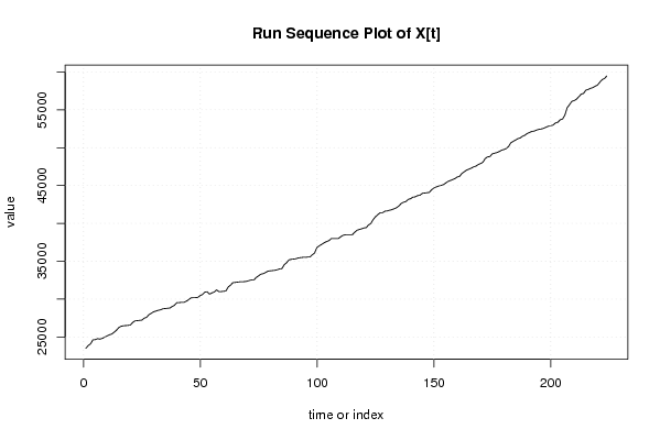
| Dataseries X: | |||||||||||||||||||||||||||||||||||||||||||||||||||||||||||||||||
23500.89 23870.25 24087.04 24617.61 24649 24774.76 24711.84 24806.25 24964 25122.25 25281 25376.49 25600 25856.64 26211.61 26406.25 26471.29 26503.84 26536.41 26569 26896 27126.09 27159.04 27192.01 27225 27489.64 27589.21 27955.84 28123.29 28324.89 28425.96 28527.21 28594.81 28730.25 28764.16 28798.09 28832.04 29036.16 29206.81 29549.61 29549.61 29584 29584 29721.76 29929 30171.69 30206.44 30206.44 30241.21 30485.16 30625 30940.81 30976 30660.01 30835.36 30940.81 31222.89 31011.21 31011.21 31046.44 31081.69 31612.84 31862.25 32184.36 32220.25 32256.16 32292.09 32292.09 32328.04 32364.01 32472.04 32544.16 32544.16 32869.69 33087.61 33306.25 33379.29 33525.61 33708.96 33745.69 33782.44 33819.21 33892.81 34003.36 34040.25 34558.81 34819.56 35193.76 35268.84 35306.41 35344 35456.89 35494.56 35532.25 35532.25 35569.96 35569.96 35872.36 36100 36825.61 37056.25 37249 37442.25 37597.21 37713.64 37986.01 37986.01 37986.01 37986.01 38220.25 38416 38494.44 38494.44 38494.44 38494.44 38809 39085.29 39204 39283.24 39402.25 39441.96 39800.25 40000 40521.69 40884.84 41168.41 41412.25 41412.25 41616 41656.81 41738.49 41820.25 41943.04 42066.01 42312.49 42642.25 42807.61 42890.41 43180.84 43264 43472.25 43513.96 43681 43722.81 43974.09 44016.04 44058.01 44100 44436.64 44689.96 44816.89 44944 45028.84 45113.76 45326.41 45539.56 45667.69 45796 45924.49 46139.04 46225 46612.81 46828.96 47045.61 47175.84 47306.25 47480.41 47567.61 47785.96 47917.21 48092.49 48576.16 48796.81 48841 49195.24 49284 49372.84 49506.25 49684.41 49773.61 49907.56 50176 50670.01 50850.25 51030.81 51211.69 51302.25 51529 51665.29 51892.84 52029.61 52166.56 52212.25 52349.44 52441 52486.81 52578.49 52716.16 52854.01 52900 52992.04 53268.64 53361 53684.89 53777.61 54289 55272.01 55696 56121.61 56216.41 56406.25 56739.24 57073.21 57168.81 57600 57696.04 57840.25 57936.49 58129.21 58273.96 58660.84 59000.41 59146.24 59487.21 | |||||||||||||||||||||||||||||||||||||||||||||||||||||||||||||||||
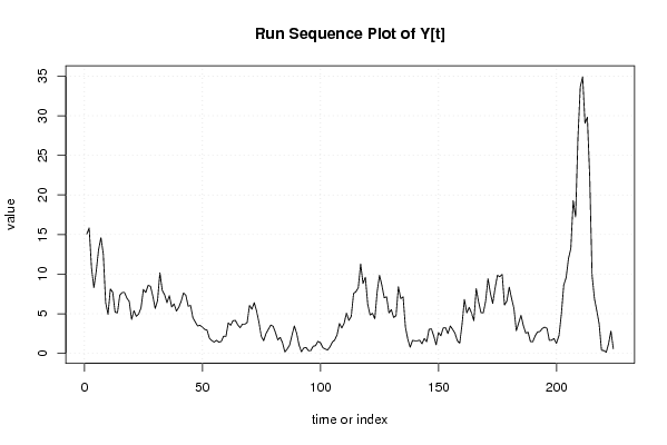
| Dataseries Y: | |||||||||||||||||||||||||||||||||||||||||||||||||||||||||||||||||
15.0544 15.8404 10.8241 8.2944 10.3684 13.1044 14.5924 12.5316 6.4009 4.9284 8.1225 7.7284 5.1984 5.1076 7.3441 7.6729 7.6729 6.9696 6.5536 4.2849 5.3824 4.6656 4.9729 5.76 8.0656 7.6729 8.5849 8.4681 7.2361 5.6644 6.6564 10.1761 7.9524 7.3984 6.4009 7.29 5.8564 6.25 5.3361 5.8081 6.5536 7.6176 7.3441 5.9536 6.0516 4.4944 3.9601 3.4596 3.5344 3.3124 3.0276 2.9241 1.9044 1.6129 1.4161 1.6384 1.4161 1.4884 2.1609 2.1316 3.8416 3.5344 4.1209 4.1616 3.61 3.24 3.6864 3.6864 3.8809 6.0516 5.5696 6.4009 5.3361 3.9204 2.1316 1.5876 2.4964 3.0276 3.5721 3.4225 2.6244 1.69 2.0164 1.3225 0.1764 0.5476 1.0404 2.2801 3.4596 2.5281 1.0609 0.1936 0.6724 0.7396 0.3364 0.3481 0.9025 0.9604 1.5129 1.3689 0.7056 0.5476 0.4225 0.8281 1.4161 1.69 2.3409 3.7636 3.2041 3.8025 5.1076 4.1616 4.6656 7.5625 7.7841 8.2944 11.2896 8.8209 9.61 6.2001 4.84 5.0625 4.3681 7.7841 9.8596 8.5849 7.0225 7.1289 5.1076 5.5225 4.5369 4.7524 8.41 6.9169 7.1289 3.2761 1.7689 0.7744 1.6384 1.5876 1.5876 1.6641 1.21 1.8769 1.4641 3.0276 3.0976 2.1904 1.0816 2.6244 2.2201 3.2041 3.24 2.4964 3.4596 3.0276 2.5281 1.5876 1.2769 3.6864 6.8121 5.1076 5.8081 5.1076 4.1209 8.1796 6.5025 5.1529 5.1076 6.6049 9.4249 7.6176 6.3001 8.2369 9.8596 9.6721 9.9856 6.1009 6.6049 8.3521 6.9169 5.6644 2.8561 3.8416 4.7961 3.4969 2.56 2.6569 1.4884 1.4641 2.2201 2.6896 2.7556 3.1329 3.3124 3.1684 1.6384 1.6641 1.8769 1.2544 2.2801 5.0176 8.6436 9.5481 11.9716 13.2496 19.2721 17.2225 27.1441 33.64 34.9281 29.0521 29.8116 22.2784 9.8596 6.9169 5.3824 3.7249 0.3844 0.36 0.1369 1.21 2.8224 0.6084 | |||||||||||||||||||||||||||||||||||||||||||||||||||||||||||||||||
Tables (Output of Computation) | |||||||||||||||||||||||||||||||||||||||||||||||||||||||||||||||||
| |||||||||||||||||||||||||||||||||||||||||||||||||||||||||||||||||
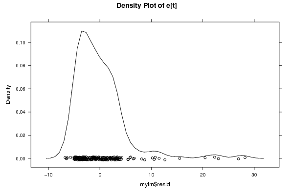
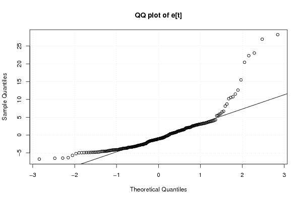
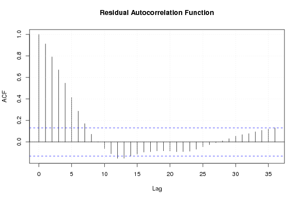
Figures (Output of Computation) | |||||||||||||||||||||||||||||||||||||||||||||||||||||||||||||||||
Input Parameters & R Code | |||||||||||||||||||||||||||||||||||||||||||||||||||||||||||||||||
| Parameters (Session): | |||||||||||||||||||||||||||||||||||||||||||||||||||||||||||||||||
| par1 = 0 ; par2 = 36 ; | |||||||||||||||||||||||||||||||||||||||||||||||||||||||||||||||||
| Parameters (R input): | |||||||||||||||||||||||||||||||||||||||||||||||||||||||||||||||||
| par1 = 0 ; par2 = 36 ; | |||||||||||||||||||||||||||||||||||||||||||||||||||||||||||||||||
| R code (references can be found in the software module): | |||||||||||||||||||||||||||||||||||||||||||||||||||||||||||||||||
par1 <- as.numeric(par1) | |||||||||||||||||||||||||||||||||||||||||||||||||||||||||||||||||