Repository of Reproducible Computations

Free Statistics

of Irreproducible Research!

Author's title

Author

*Unverified author*

R Software Module

rwasp_autocorrelation.wasp

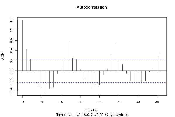
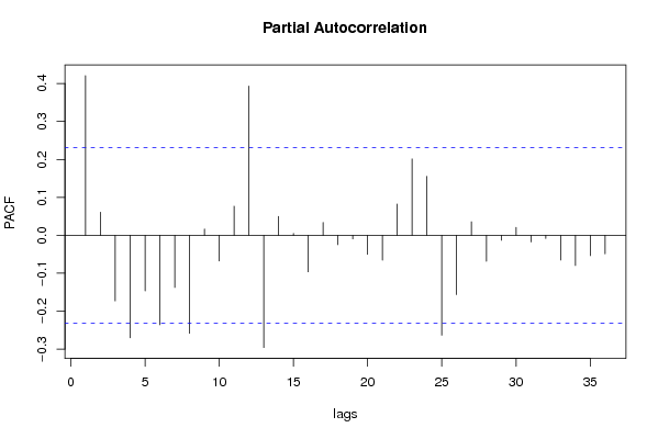
Title produced by software

(Partial) Autocorrelation Function

Date of computation

Fri, 27 Nov 2009 09:33:53 -0700

Cite this page as follows

Statistical Computations at FreeStatistics.org, Office for Research Development and Education, URL https://freestatistics.org/blog/index.php?v=date/2009/Nov/27/t1259339707qzs69rhr1qgwjms.htm/, Retrieved Mon, 29 Apr 2024 04:56:13 +0000

Statistical Computations at FreeStatistics.org, Office for Research Development and Education, URL https://freestatistics.org/blog/index.php?pk=60964, Retrieved Mon, 29 Apr 2024 04:56:13 +0000

QR Codes:

Paste this QR Code to cite your computation.

Original text written by user:

IsPrivate?

No (this computation is public)

User-defined keywords

Estimated Impact

133

Family? (F = Feedback message, R = changed R code, M = changed R Module, P = changed Parameters, D = changed Data)

-       [(Partial) Autocorrelation Function] [] [2009-11-27 16:33:53] [8803431e497d94425e57d35981fe4f1d] [Current]
-   P     [(Partial) Autocorrelation Function] [] [2009-11-27 16:43:06] [898d317f4f946fbfcc4d07699283d43b] 
-   P     [(Partial) Autocorrelation Function] [] [2009-11-27 16:47:12] [898d317f4f946fbfcc4d07699283d43b] 
- RMP     [Variance Reduction Matrix] [] [2009-11-27 17:11:01] [898d317f4f946fbfcc4d07699283d43b] 
- RMP     [Spectral Analysis] [] [2009-11-27 17:24:08] [a8dc04902f2584d6dc8a82e937850322] 
- RMP     [Spectral Analysis] [] [2009-11-27 17:29:20] [a8dc04902f2584d6dc8a82e937850322] 
- RMP     [Spectral Analysis] [] [2009-11-27 17:32:58] [a8dc04902f2584d6dc8a82e937850322] 
- RMP     [Standard Deviation-Mean Plot] [] [2009-11-27 17:40:19] [a8dc04902f2584d6dc8a82e937850322] 

Feedback Forum

Post a new message

Dataseries X:

Download CSV

Histogram

Boxplots

Summary of computational transaction
Raw Input	view raw input (R code)
Raw Output	view raw output of R engine
Computing time	1 seconds
R Server	'Gwilym Jenkins' @ 72.249.127.135

\begin{tabular}{lllllllll}
\hline
Summary of computational transaction \tabularnewline
Raw Input & view raw input (R code)  \tabularnewline
Raw Output & view raw output of R engine  \tabularnewline
Computing time & 1 seconds \tabularnewline
R Server & 'Gwilym Jenkins' @ 72.249.127.135 \tabularnewline
\hline
\end{tabular}
%Source: https://freestatistics.org/blog/index.php?pk=60964&T=0

[TABLE]
[ROW][C]Summary of computational transaction[/C][/ROW]
[ROW][C]Raw Input[/C][C]view raw input (R code) [/C][/ROW]
[ROW][C]Raw Output[/C][C]view raw output of R engine [/C][/ROW]
[ROW][C]Computing time[/C][C]1 seconds[/C][/ROW]
[ROW][C]R Server[/C][C]'Gwilym Jenkins' @ 72.249.127.135[/C][/ROW]
[/TABLE]
Source: https://freestatistics.org/blog/index.php?pk=60964&T=0

Globally Unique Identifier (entire table): ba.freestatistics.org/blog/index.php?pk=60964&T=0

As an alternative you can also use a QR Code:

The GUIDs for individual cells are displayed in the table below:

Summary of computational transaction
Raw Input	view raw input (R code)
Raw Output	view raw output of R engine
Computing time	1 seconds
R Server	'Gwilym Jenkins' @ 72.249.127.135

Autocorrelation Function
Time lag k	ACF(k)	T-STAT	P-value
1	0.420701	3.5698	0.00032
2	0.227057	1.9266	0.028986
3	-0.026365	-0.2237	0.411806
4	-0.269141	-2.2837	0.01267
5	-0.337099	-2.8604	0.002767
6	-0.429438	-3.6439	0.000252
7	-0.348298	-2.9554	0.002109
8	-0.326429	-2.7698	0.003565
9	-0.05789	-0.4912	0.312384
10	0.081015	0.6874	0.247007
11	0.282198	2.3945	0.009623
12	0.591205	5.0165	2e-06
13	0.248793	2.1111	0.019119
14	0.237259	2.0132	0.023916
15	0.031822	0.27	0.393959
16	-0.16458	-1.3965	0.083426
17	-0.226267	-1.9199	0.029414
18	-0.312358	-2.6504	0.004939
19	-0.264632	-2.2455	0.013904
20	-0.27992	-2.3752	0.010102
21	-0.077005	-0.6534	0.257786
22	0.04203	0.3566	0.361204
23	0.322896	2.7399	0.003872
24	0.528329	4.483	1.4e-05
25	0.161095	1.3669	0.087949
26	0.126988	1.0775	0.14242
27	-0.051806	-0.4396	0.330776
28	-0.198388	-1.6834	0.048317
29	-0.22807	-1.9352	0.028444
30	-0.262828	-2.2302	0.014427
31	-0.211671	-1.7961	0.038338
32	-0.196476	-1.6672	0.049914
33	-0.019074	-0.1618	0.435939
34	0.037347	0.3169	0.376119
35	0.259394	2.201	0.01547
36	0.358348	3.0407	0.001645

\begin{tabular}{lllllllll}
\hline
Autocorrelation Function \tabularnewline
Time lag k & ACF(k) & T-STAT & P-value \tabularnewline
1 & 0.420701 & 3.5698 & 0.00032 \tabularnewline
2 & 0.227057 & 1.9266 & 0.028986 \tabularnewline
3 & -0.026365 & -0.2237 & 0.411806 \tabularnewline
4 & -0.269141 & -2.2837 & 0.01267 \tabularnewline
5 & -0.337099 & -2.8604 & 0.002767 \tabularnewline
6 & -0.429438 & -3.6439 & 0.000252 \tabularnewline
7 & -0.348298 & -2.9554 & 0.002109 \tabularnewline
8 & -0.326429 & -2.7698 & 0.003565 \tabularnewline
9 & -0.05789 & -0.4912 & 0.312384 \tabularnewline
10 & 0.081015 & 0.6874 & 0.247007 \tabularnewline
11 & 0.282198 & 2.3945 & 0.009623 \tabularnewline
12 & 0.591205 & 5.0165 & 2e-06 \tabularnewline
13 & 0.248793 & 2.1111 & 0.019119 \tabularnewline
14 & 0.237259 & 2.0132 & 0.023916 \tabularnewline
15 & 0.031822 & 0.27 & 0.393959 \tabularnewline
16 & -0.16458 & -1.3965 & 0.083426 \tabularnewline
17 & -0.226267 & -1.9199 & 0.029414 \tabularnewline
18 & -0.312358 & -2.6504 & 0.004939 \tabularnewline
19 & -0.264632 & -2.2455 & 0.013904 \tabularnewline
20 & -0.27992 & -2.3752 & 0.010102 \tabularnewline
21 & -0.077005 & -0.6534 & 0.257786 \tabularnewline
22 & 0.04203 & 0.3566 & 0.361204 \tabularnewline
23 & 0.322896 & 2.7399 & 0.003872 \tabularnewline
24 & 0.528329 & 4.483 & 1.4e-05 \tabularnewline
25 & 0.161095 & 1.3669 & 0.087949 \tabularnewline
26 & 0.126988 & 1.0775 & 0.14242 \tabularnewline
27 & -0.051806 & -0.4396 & 0.330776 \tabularnewline
28 & -0.198388 & -1.6834 & 0.048317 \tabularnewline
29 & -0.22807 & -1.9352 & 0.028444 \tabularnewline
30 & -0.262828 & -2.2302 & 0.014427 \tabularnewline
31 & -0.211671 & -1.7961 & 0.038338 \tabularnewline
32 & -0.196476 & -1.6672 & 0.049914 \tabularnewline
33 & -0.019074 & -0.1618 & 0.435939 \tabularnewline
34 & 0.037347 & 0.3169 & 0.376119 \tabularnewline
35 & 0.259394 & 2.201 & 0.01547 \tabularnewline
36 & 0.358348 & 3.0407 & 0.001645 \tabularnewline
\hline
\end{tabular}
%Source: https://freestatistics.org/blog/index.php?pk=60964&T=1

[TABLE]
[ROW][C]Autocorrelation Function[/C][/ROW]
[ROW][C]Time lag k[/C][C]ACF(k)[/C][C]T-STAT[/C][C]P-value[/C][/ROW]
[ROW][C]1[/C][C]0.420701[/C][C]3.5698[/C][C]0.00032[/C][/ROW]
[ROW][C]2[/C][C]0.227057[/C][C]1.9266[/C][C]0.028986[/C][/ROW]
[ROW][C]3[/C][C]-0.026365[/C][C]-0.2237[/C][C]0.411806[/C][/ROW]
[ROW][C]4[/C][C]-0.269141[/C][C]-2.2837[/C][C]0.01267[/C][/ROW]
[ROW][C]5[/C][C]-0.337099[/C][C]-2.8604[/C][C]0.002767[/C][/ROW]
[ROW][C]6[/C][C]-0.429438[/C][C]-3.6439[/C][C]0.000252[/C][/ROW]
[ROW][C]7[/C][C]-0.348298[/C][C]-2.9554[/C][C]0.002109[/C][/ROW]
[ROW][C]8[/C][C]-0.326429[/C][C]-2.7698[/C][C]0.003565[/C][/ROW]
[ROW][C]9[/C][C]-0.05789[/C][C]-0.4912[/C][C]0.312384[/C][/ROW]
[ROW][C]10[/C][C]0.081015[/C][C]0.6874[/C][C]0.247007[/C][/ROW]
[ROW][C]11[/C][C]0.282198[/C][C]2.3945[/C][C]0.009623[/C][/ROW]
[ROW][C]12[/C][C]0.591205[/C][C]5.0165[/C][C]2e-06[/C][/ROW]
[ROW][C]13[/C][C]0.248793[/C][C]2.1111[/C][C]0.019119[/C][/ROW]
[ROW][C]14[/C][C]0.237259[/C][C]2.0132[/C][C]0.023916[/C][/ROW]
[ROW][C]15[/C][C]0.031822[/C][C]0.27[/C][C]0.393959[/C][/ROW]
[ROW][C]16[/C][C]-0.16458[/C][C]-1.3965[/C][C]0.083426[/C][/ROW]
[ROW][C]17[/C][C]-0.226267[/C][C]-1.9199[/C][C]0.029414[/C][/ROW]
[ROW][C]18[/C][C]-0.312358[/C][C]-2.6504[/C][C]0.004939[/C][/ROW]
[ROW][C]19[/C][C]-0.264632[/C][C]-2.2455[/C][C]0.013904[/C][/ROW]
[ROW][C]20[/C][C]-0.27992[/C][C]-2.3752[/C][C]0.010102[/C][/ROW]
[ROW][C]21[/C][C]-0.077005[/C][C]-0.6534[/C][C]0.257786[/C][/ROW]
[ROW][C]22[/C][C]0.04203[/C][C]0.3566[/C][C]0.361204[/C][/ROW]
[ROW][C]23[/C][C]0.322896[/C][C]2.7399[/C][C]0.003872[/C][/ROW]
[ROW][C]24[/C][C]0.528329[/C][C]4.483[/C][C]1.4e-05[/C][/ROW]
[ROW][C]25[/C][C]0.161095[/C][C]1.3669[/C][C]0.087949[/C][/ROW]
[ROW][C]26[/C][C]0.126988[/C][C]1.0775[/C][C]0.14242[/C][/ROW]
[ROW][C]27[/C][C]-0.051806[/C][C]-0.4396[/C][C]0.330776[/C][/ROW]
[ROW][C]28[/C][C]-0.198388[/C][C]-1.6834[/C][C]0.048317[/C][/ROW]
[ROW][C]29[/C][C]-0.22807[/C][C]-1.9352[/C][C]0.028444[/C][/ROW]
[ROW][C]30[/C][C]-0.262828[/C][C]-2.2302[/C][C]0.014427[/C][/ROW]
[ROW][C]31[/C][C]-0.211671[/C][C]-1.7961[/C][C]0.038338[/C][/ROW]
[ROW][C]32[/C][C]-0.196476[/C][C]-1.6672[/C][C]0.049914[/C][/ROW]
[ROW][C]33[/C][C]-0.019074[/C][C]-0.1618[/C][C]0.435939[/C][/ROW]
[ROW][C]34[/C][C]0.037347[/C][C]0.3169[/C][C]0.376119[/C][/ROW]
[ROW][C]35[/C][C]0.259394[/C][C]2.201[/C][C]0.01547[/C][/ROW]
[ROW][C]36[/C][C]0.358348[/C][C]3.0407[/C][C]0.001645[/C][/ROW]
[/TABLE]
Source: https://freestatistics.org/blog/index.php?pk=60964&T=1

Globally Unique Identifier (entire table): ba.freestatistics.org/blog/index.php?pk=60964&T=1

As an alternative you can also use a QR Code:

The GUIDs for individual cells are displayed in the table below:

Autocorrelation Function
Time lag k	ACF(k)	T-STAT	P-value
1	0.420701	3.5698	0.00032
2	0.227057	1.9266	0.028986
3	-0.026365	-0.2237	0.411806
4	-0.269141	-2.2837	0.01267
5	-0.337099	-2.8604	0.002767
6	-0.429438	-3.6439	0.000252
7	-0.348298	-2.9554	0.002109
8	-0.326429	-2.7698	0.003565
9	-0.05789	-0.4912	0.312384
10	0.081015	0.6874	0.247007
11	0.282198	2.3945	0.009623
12	0.591205	5.0165	2e-06
13	0.248793	2.1111	0.019119
14	0.237259	2.0132	0.023916
15	0.031822	0.27	0.393959
16	-0.16458	-1.3965	0.083426
17	-0.226267	-1.9199	0.029414
18	-0.312358	-2.6504	0.004939
19	-0.264632	-2.2455	0.013904
20	-0.27992	-2.3752	0.010102
21	-0.077005	-0.6534	0.257786
22	0.04203	0.3566	0.361204
23	0.322896	2.7399	0.003872
24	0.528329	4.483	1.4e-05
25	0.161095	1.3669	0.087949
26	0.126988	1.0775	0.14242
27	-0.051806	-0.4396	0.330776
28	-0.198388	-1.6834	0.048317
29	-0.22807	-1.9352	0.028444
30	-0.262828	-2.2302	0.014427
31	-0.211671	-1.7961	0.038338
32	-0.196476	-1.6672	0.049914
33	-0.019074	-0.1618	0.435939
34	0.037347	0.3169	0.376119
35	0.259394	2.201	0.01547
36	0.358348	3.0407	0.001645

Partial Autocorrelation Function
Time lag k	PACF(k)	T-STAT	P-value
1	0.420701	3.5698	0.00032
2	0.060835	0.5162	0.303648
3	-0.172776	-1.4661	0.073493
4	-0.270365	-2.2941	0.012351
5	-0.146616	-1.2441	0.108753
6	-0.235724	-2.0002	0.024626
7	-0.137322	-1.1652	0.123889
8	-0.258259	-2.1914	0.01583
9	0.016646	0.1412	0.444034
10	-0.067662	-0.5741	0.283836
11	0.076724	0.651	0.258552
12	0.393171	3.3362	0.000673
13	-0.295759	-2.5096	0.007168
14	0.049811	0.4227	0.3369
15	0.004813	0.0408	0.483767
16	-0.096384	-0.8178	0.208072
17	0.03371	0.286	0.387836
18	-0.024883	-0.2111	0.416686
19	-0.009628	-0.0817	0.467558
20	-0.050477	-0.4283	0.334853
21	-0.065582	-0.5565	0.289803
22	0.082337	0.6987	0.24351
23	0.201178	1.7071	0.046061
24	0.155191	1.3168	0.096035
25	-0.263494	-2.2358	0.014232
26	-0.156145	-1.3249	0.094691
27	0.035647	0.3025	0.38158
28	-0.068624	-0.5823	0.281094
29	-0.013122	-0.1113	0.455828
30	0.02072	0.1758	0.430467
31	-0.017313	-0.1469	0.441809
32	-0.008375	-0.0711	0.471772
33	-0.065019	-0.5517	0.291429
34	-0.079665	-0.676	0.250611
35	-0.053647	-0.4552	0.325165
36	-0.04897	-0.4155	0.339496

\begin{tabular}{lllllllll}
\hline
Partial Autocorrelation Function \tabularnewline
Time lag k & PACF(k) & T-STAT & P-value \tabularnewline
1 & 0.420701 & 3.5698 & 0.00032 \tabularnewline
2 & 0.060835 & 0.5162 & 0.303648 \tabularnewline
3 & -0.172776 & -1.4661 & 0.073493 \tabularnewline
4 & -0.270365 & -2.2941 & 0.012351 \tabularnewline
5 & -0.146616 & -1.2441 & 0.108753 \tabularnewline
6 & -0.235724 & -2.0002 & 0.024626 \tabularnewline
7 & -0.137322 & -1.1652 & 0.123889 \tabularnewline
8 & -0.258259 & -2.1914 & 0.01583 \tabularnewline
9 & 0.016646 & 0.1412 & 0.444034 \tabularnewline
10 & -0.067662 & -0.5741 & 0.283836 \tabularnewline
11 & 0.076724 & 0.651 & 0.258552 \tabularnewline
12 & 0.393171 & 3.3362 & 0.000673 \tabularnewline
13 & -0.295759 & -2.5096 & 0.007168 \tabularnewline
14 & 0.049811 & 0.4227 & 0.3369 \tabularnewline
15 & 0.004813 & 0.0408 & 0.483767 \tabularnewline
16 & -0.096384 & -0.8178 & 0.208072 \tabularnewline
17 & 0.03371 & 0.286 & 0.387836 \tabularnewline
18 & -0.024883 & -0.2111 & 0.416686 \tabularnewline
19 & -0.009628 & -0.0817 & 0.467558 \tabularnewline
20 & -0.050477 & -0.4283 & 0.334853 \tabularnewline
21 & -0.065582 & -0.5565 & 0.289803 \tabularnewline
22 & 0.082337 & 0.6987 & 0.24351 \tabularnewline
23 & 0.201178 & 1.7071 & 0.046061 \tabularnewline
24 & 0.155191 & 1.3168 & 0.096035 \tabularnewline
25 & -0.263494 & -2.2358 & 0.014232 \tabularnewline
26 & -0.156145 & -1.3249 & 0.094691 \tabularnewline
27 & 0.035647 & 0.3025 & 0.38158 \tabularnewline
28 & -0.068624 & -0.5823 & 0.281094 \tabularnewline
29 & -0.013122 & -0.1113 & 0.455828 \tabularnewline
30 & 0.02072 & 0.1758 & 0.430467 \tabularnewline
31 & -0.017313 & -0.1469 & 0.441809 \tabularnewline
32 & -0.008375 & -0.0711 & 0.471772 \tabularnewline
33 & -0.065019 & -0.5517 & 0.291429 \tabularnewline
34 & -0.079665 & -0.676 & 0.250611 \tabularnewline
35 & -0.053647 & -0.4552 & 0.325165 \tabularnewline
36 & -0.04897 & -0.4155 & 0.339496 \tabularnewline
\hline
\end{tabular}
%Source: https://freestatistics.org/blog/index.php?pk=60964&T=2

[TABLE]
[ROW][C]Partial Autocorrelation Function[/C][/ROW]
[ROW][C]Time lag k[/C][C]PACF(k)[/C][C]T-STAT[/C][C]P-value[/C][/ROW]
[ROW][C]1[/C][C]0.420701[/C][C]3.5698[/C][C]0.00032[/C][/ROW]
[ROW][C]2[/C][C]0.060835[/C][C]0.5162[/C][C]0.303648[/C][/ROW]
[ROW][C]3[/C][C]-0.172776[/C][C]-1.4661[/C][C]0.073493[/C][/ROW]
[ROW][C]4[/C][C]-0.270365[/C][C]-2.2941[/C][C]0.012351[/C][/ROW]
[ROW][C]5[/C][C]-0.146616[/C][C]-1.2441[/C][C]0.108753[/C][/ROW]
[ROW][C]6[/C][C]-0.235724[/C][C]-2.0002[/C][C]0.024626[/C][/ROW]
[ROW][C]7[/C][C]-0.137322[/C][C]-1.1652[/C][C]0.123889[/C][/ROW]
[ROW][C]8[/C][C]-0.258259[/C][C]-2.1914[/C][C]0.01583[/C][/ROW]
[ROW][C]9[/C][C]0.016646[/C][C]0.1412[/C][C]0.444034[/C][/ROW]
[ROW][C]10[/C][C]-0.067662[/C][C]-0.5741[/C][C]0.283836[/C][/ROW]
[ROW][C]11[/C][C]0.076724[/C][C]0.651[/C][C]0.258552[/C][/ROW]
[ROW][C]12[/C][C]0.393171[/C][C]3.3362[/C][C]0.000673[/C][/ROW]
[ROW][C]13[/C][C]-0.295759[/C][C]-2.5096[/C][C]0.007168[/C][/ROW]
[ROW][C]14[/C][C]0.049811[/C][C]0.4227[/C][C]0.3369[/C][/ROW]
[ROW][C]15[/C][C]0.004813[/C][C]0.0408[/C][C]0.483767[/C][/ROW]
[ROW][C]16[/C][C]-0.096384[/C][C]-0.8178[/C][C]0.208072[/C][/ROW]
[ROW][C]17[/C][C]0.03371[/C][C]0.286[/C][C]0.387836[/C][/ROW]
[ROW][C]18[/C][C]-0.024883[/C][C]-0.2111[/C][C]0.416686[/C][/ROW]
[ROW][C]19[/C][C]-0.009628[/C][C]-0.0817[/C][C]0.467558[/C][/ROW]
[ROW][C]20[/C][C]-0.050477[/C][C]-0.4283[/C][C]0.334853[/C][/ROW]
[ROW][C]21[/C][C]-0.065582[/C][C]-0.5565[/C][C]0.289803[/C][/ROW]
[ROW][C]22[/C][C]0.082337[/C][C]0.6987[/C][C]0.24351[/C][/ROW]
[ROW][C]23[/C][C]0.201178[/C][C]1.7071[/C][C]0.046061[/C][/ROW]
[ROW][C]24[/C][C]0.155191[/C][C]1.3168[/C][C]0.096035[/C][/ROW]
[ROW][C]25[/C][C]-0.263494[/C][C]-2.2358[/C][C]0.014232[/C][/ROW]
[ROW][C]26[/C][C]-0.156145[/C][C]-1.3249[/C][C]0.094691[/C][/ROW]
[ROW][C]27[/C][C]0.035647[/C][C]0.3025[/C][C]0.38158[/C][/ROW]
[ROW][C]28[/C][C]-0.068624[/C][C]-0.5823[/C][C]0.281094[/C][/ROW]
[ROW][C]29[/C][C]-0.013122[/C][C]-0.1113[/C][C]0.455828[/C][/ROW]
[ROW][C]30[/C][C]0.02072[/C][C]0.1758[/C][C]0.430467[/C][/ROW]
[ROW][C]31[/C][C]-0.017313[/C][C]-0.1469[/C][C]0.441809[/C][/ROW]
[ROW][C]32[/C][C]-0.008375[/C][C]-0.0711[/C][C]0.471772[/C][/ROW]
[ROW][C]33[/C][C]-0.065019[/C][C]-0.5517[/C][C]0.291429[/C][/ROW]
[ROW][C]34[/C][C]-0.079665[/C][C]-0.676[/C][C]0.250611[/C][/ROW]
[ROW][C]35[/C][C]-0.053647[/C][C]-0.4552[/C][C]0.325165[/C][/ROW]
[ROW][C]36[/C][C]-0.04897[/C][C]-0.4155[/C][C]0.339496[/C][/ROW]
[/TABLE]
Source: https://freestatistics.org/blog/index.php?pk=60964&T=2

Globally Unique Identifier (entire table): ba.freestatistics.org/blog/index.php?pk=60964&T=2

As an alternative you can also use a QR Code:

The GUIDs for individual cells are displayed in the table below:

Partial Autocorrelation Function
Time lag k	PACF(k)	T-STAT	P-value
1	0.420701	3.5698	0.00032
2	0.060835	0.5162	0.303648
3	-0.172776	-1.4661	0.073493
4	-0.270365	-2.2941	0.012351
5	-0.146616	-1.2441	0.108753
6	-0.235724	-2.0002	0.024626
7	-0.137322	-1.1652	0.123889
8	-0.258259	-2.1914	0.01583
9	0.016646	0.1412	0.444034
10	-0.067662	-0.5741	0.283836
11	0.076724	0.651	0.258552
12	0.393171	3.3362	0.000673
13	-0.295759	-2.5096	0.007168
14	0.049811	0.4227	0.3369
15	0.004813	0.0408	0.483767
16	-0.096384	-0.8178	0.208072
17	0.03371	0.286	0.387836
18	-0.024883	-0.2111	0.416686
19	-0.009628	-0.0817	0.467558
20	-0.050477	-0.4283	0.334853
21	-0.065582	-0.5565	0.289803
22	0.082337	0.6987	0.24351
23	0.201178	1.7071	0.046061
24	0.155191	1.3168	0.096035
25	-0.263494	-2.2358	0.014232
26	-0.156145	-1.3249	0.094691
27	0.035647	0.3025	0.38158
28	-0.068624	-0.5823	0.281094
29	-0.013122	-0.1113	0.455828
30	0.02072	0.1758	0.430467
31	-0.017313	-0.1469	0.441809
32	-0.008375	-0.0711	0.471772
33	-0.065019	-0.5517	0.291429
34	-0.079665	-0.676	0.250611
35	-0.053647	-0.4552	0.325165
36	-0.04897	-0.4155	0.339496

Figure 1

PNG link

Postscript link

PDF link

Figure 2

PNG link

Postscript link

PDF link

Parameters (Session):

par1 = 36 ; par2 = 1 ; par3 = 0 ; par4 = 0 ; par5 = 12 ; par6 = White Noise ; par7 = 0.95 ;

Parameters (R input):

par1 = 36 ; par2 = 1 ; par3 = 0 ; par4 = 0 ; par5 = 12 ; par6 = White Noise ; par7 = 0.95 ;

R code (references can be found in the software module):

if (par1 == 'Default') {
par1 = 10*log10(length(x))
} else {
par1 <- as.numeric(par1)
}
par2 <- as.numeric(par2)
par3 <- as.numeric(par3)
par4 <- as.numeric(par4)
par5 <- as.numeric(par5)
if (par6 == 'White Noise') par6 <- 'white' else par6 <- 'ma'
par7 <- as.numeric(par7)
if (par2 == 0) {
x <- log(x)
} else {
x <- (x ^ par2 - 1) / par2
}
if (par3 > 0) x <- diff(x,lag=1,difference=par3)
if (par4 > 0) x <- diff(x,lag=par5,difference=par4)
bitmap(file='pic1.png')
racf <- acf(x, par1, main='Autocorrelation', xlab='time lag', ylab='ACF', ci.type=par6, ci=par7, sub=paste('(lambda=',par2,', d=',par3,', D=',par4,', CI=', par7, ', CI type=',par6,')',sep=''))
dev.off()
bitmap(file='pic2.png')
rpacf <- pacf(x,par1,main='Partial Autocorrelation',xlab='lags',ylab='PACF')
dev.off()
(myacf <- c(racf$acf))
(mypacf <- c(rpacf$acf))
lengthx <- length(x)
sqrtn <- sqrt(lengthx)
load(file='createtable')
a<-table.start()
a<-table.row.start(a)
a<-table.element(a,'Autocorrelation Function',4,TRUE)
a<-table.row.end(a)
a<-table.row.start(a)
a<-table.element(a,'Time lag k',header=TRUE)
a<-table.element(a,hyperlink('basics.htm','ACF(k)','click here for more information about the Autocorrelation Function'),header=TRUE)
a<-table.element(a,'T-STAT',header=TRUE)
a<-table.element(a,'P-value',header=TRUE)
a<-table.row.end(a)
for (i in 2:(par1+1)) {
a<-table.row.start(a)
a<-table.element(a,i-1,header=TRUE)
a<-table.element(a,round(myacf[i],6))
mytstat <- myacf[i]*sqrtn
a<-table.element(a,round(mytstat,4))
a<-table.element(a,round(1-pt(abs(mytstat),lengthx),6))
a<-table.row.end(a)
}
a<-table.end(a)
table.save(a,file='mytable.tab')
a<-table.start()
a<-table.row.start(a)
a<-table.element(a,'Partial Autocorrelation Function',4,TRUE)
a<-table.row.end(a)
a<-table.row.start(a)
a<-table.element(a,'Time lag k',header=TRUE)
a<-table.element(a,hyperlink('basics.htm','PACF(k)','click here for more information about the Partial Autocorrelation Function'),header=TRUE)
a<-table.element(a,'T-STAT',header=TRUE)
a<-table.element(a,'P-value',header=TRUE)
a<-table.row.end(a)
for (i in 1:par1) {
a<-table.row.start(a)
a<-table.element(a,i,header=TRUE)
a<-table.element(a,round(mypacf[i],6))
mytstat <- mypacf[i]*sqrtn
a<-table.element(a,round(mytstat,4))
a<-table.element(a,round(1-pt(abs(mytstat),lengthx),6))
a<-table.row.end(a)
}
a<-table.end(a)
table.save(a,file='mytable1.tab')

Free Statistics

Description of Statistical Computation

Tree of Dependent Computations

Dataset

Tables (Output of Computation)

Figures (Output of Computation)

Input Parameters & R Code