Repository of Reproducible Computations

Free Statistics

of Irreproducible Research!

Author's title

Author

*The author of this computation has been verified*

R Software Module

rwasp_edauni.wasp

Title produced by software

Univariate Explorative Data Analysis

Date of computation

Mon, 19 Oct 2009 11:59:53 -0600

Cite this page as follows

Statistical Computations at FreeStatistics.org, Office for Research Development and Education, URL https://freestatistics.org/blog/index.php?v=date/2009/Oct/19/t1255975288xewrq8976lmrvoh.htm/, Retrieved Mon, 29 Apr 2024 19:55:03 +0000

Statistical Computations at FreeStatistics.org, Office for Research Development and Education, URL https://freestatistics.org/blog/index.php?pk=48023, Retrieved Mon, 29 Apr 2024 19:55:03 +0000

QR Codes:

Paste this QR Code to cite your computation.

Original text written by user:

IsPrivate?

No (this computation is public)

User-defined keywords

Estimated Impact

118

Family? (F = Feedback message, R = changed R code, M = changed R Module, P = changed Parameters, D = changed Data)

-     [Bivariate Data Series] [Bivariate dataset] [2008-01-05 23:51:08] [74be16979710d4c4e7c6647856088456]
F RMPD  [Univariate Explorative Data Analysis] [Colombia Coffee] [2008-01-07 14:21:11] [74be16979710d4c4e7c6647856088456]
F RMPD    [Univariate Data Series] [] [2009-10-14 08:30:28] [74be16979710d4c4e7c6647856088456]
- RMP       [Central Tendency] [central tendency] [2009-10-17 11:29:28] [f7fc9270f813d017f9fa5b506fdc7682]
-    D        [Central Tendency] [WS 3 Part 2 Y[t]/...] [2009-10-19 17:32:48] [83058a88a37d754675a5cd22dab372fc]
- RMPD          [Univariate Data Series] [WS 3 Part 2 e[t] ...] [2009-10-19 17:45:14] [83058a88a37d754675a5cd22dab372fc]
- RMP               [Univariate Explorative Data Analysis] [WS 3 Part 3 EDA] [2009-10-19 17:59:53] [eba9f01697e64705b70041e6f338cb22] [Current]
- RMPD                [Harrell-Davis Quantiles] [WS 3 Part 3 confi...] [2009-10-19 18:14:26] [83058a88a37d754675a5cd22dab372fc] 
-   P                 [Univariate Explorative Data Analysis] [WS 3 Part 3 toevo...] [2009-10-20 18:06:02] [83058a88a37d754675a5cd22dab372fc] 
- RMP                 [Central Tendency] [WS 3 Part 3 toevo...] [2009-10-20 18:07:48] [83058a88a37d754675a5cd22dab372fc] 

Feedback Forum

Post a new message

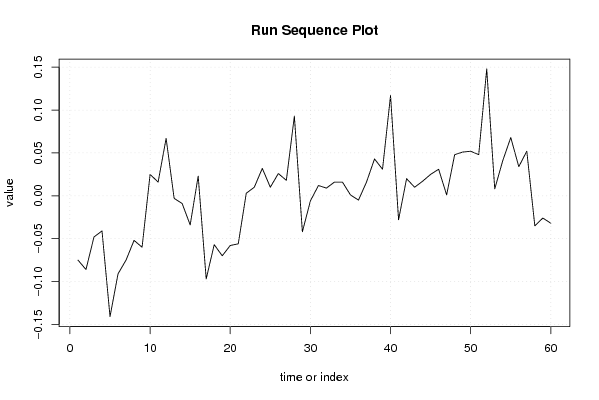
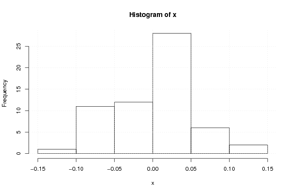
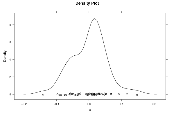
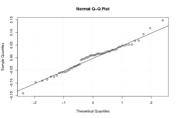
Dataseries X:

Download CSV

Histogram

Boxplots

-0.075
-0.086
-0.048
-0.041
-0.141
-0.091
-0.075
-0.052
-0.060
0.025
0.016
0.067
-0.003
-0.009
-0.034
0.023
-0.097
-0.057
-0.070
-0.058
-0.056
0.003
0.010
0.032
0.010
0.026
0.018
0.093
-0.042
-0.006
0.012
0.009
0.016
0.016
0.001
-0.005
0.016
0.043
0.031
0.117
-0.028
0.020
0.010
0.017
0.025
0.031
0.001
0.048
0.051
0.052
0.048
0.148
0.008
0.041
0.068
0.034
0.052
-0.035
-0.026
-0.032

Summary of computational transaction
Raw Input	view raw input (R code)
Raw Output	view raw output of R engine
Computing time	4 seconds
R Server	'Sir Ronald Aylmer Fisher' @ 193.190.124.24

\begin{tabular}{lllllllll}
\hline
Summary of computational transaction \tabularnewline
Raw Input & view raw input (R code)  \tabularnewline
Raw Output & view raw output of R engine  \tabularnewline
Computing time & 4 seconds \tabularnewline
R Server & 'Sir Ronald Aylmer Fisher' @ 193.190.124.24 \tabularnewline
\hline
\end{tabular}
%Source: https://freestatistics.org/blog/index.php?pk=48023&T=0

[TABLE]
[ROW][C]Summary of computational transaction[/C][/ROW]
[ROW][C]Raw Input[/C][C]view raw input (R code) [/C][/ROW]
[ROW][C]Raw Output[/C][C]view raw output of R engine [/C][/ROW]
[ROW][C]Computing time[/C][C]4 seconds[/C][/ROW]
[ROW][C]R Server[/C][C]'Sir Ronald Aylmer Fisher' @ 193.190.124.24[/C][/ROW]
[/TABLE]
Source: https://freestatistics.org/blog/index.php?pk=48023&T=0

Globally Unique Identifier (entire table): ba.freestatistics.org/blog/index.php?pk=48023&T=0

As an alternative you can also use a QR Code:

The GUIDs for individual cells are displayed in the table below:

Summary of computational transaction
Raw Input	view raw input (R code)
Raw Output	view raw output of R engine
Computing time	4 seconds
R Server	'Sir Ronald Aylmer Fisher' @ 193.190.124.24

Descriptive Statistics
# observations	60
minimum	-0.141
Q1	-0.0365
median	0.01
mean	0.000183333333333334
Q3	0.031
maximum	0.148

\begin{tabular}{lllllllll}
\hline
Descriptive Statistics \tabularnewline
# observations & 60 \tabularnewline
minimum & -0.141 \tabularnewline
Q1 & -0.0365 \tabularnewline
median & 0.01 \tabularnewline
mean & 0.000183333333333334 \tabularnewline
Q3 & 0.031 \tabularnewline
maximum & 0.148 \tabularnewline
\hline
\end{tabular}
%Source: https://freestatistics.org/blog/index.php?pk=48023&T=1

[TABLE]
[ROW][C]Descriptive Statistics[/C][/ROW]
[ROW][C]# observations[/C][C]60[/C][/ROW]
[ROW][C]minimum[/C][C]-0.141[/C][/ROW]
[ROW][C]Q1[/C][C]-0.0365[/C][/ROW]
[ROW][C]median[/C][C]0.01[/C][/ROW]
[ROW][C]mean[/C][C]0.000183333333333334[/C][/ROW]
[ROW][C]Q3[/C][C]0.031[/C][/ROW]
[ROW][C]maximum[/C][C]0.148[/C][/ROW]
[/TABLE]
Source: https://freestatistics.org/blog/index.php?pk=48023&T=1

Globally Unique Identifier (entire table): ba.freestatistics.org/blog/index.php?pk=48023&T=1

As an alternative you can also use a QR Code:

The GUIDs for individual cells are displayed in the table below:

Descriptive Statistics
# observations	60
minimum	-0.141
Q1	-0.0365
median	0.01
mean	0.000183333333333334
Q3	0.031
maximum	0.148

Figure 1

PNG link

Postscript link

PDF link

Figure 2

PNG link

Postscript link

PDF link

Figure 3

PNG link

Postscript link

PDF link

Figure 4

PNG link

Postscript link

PDF link

Figure 5

PNG link

Postscript link

PDF link

Figure 6

PNG link

Postscript link

PDF link

Figure 7

PNG link

Postscript link

PDF link

Parameters (Session):

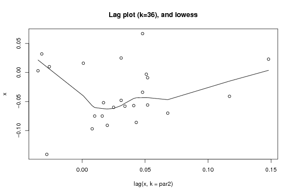
par1 = 0 ; par2 = 36 ;

Parameters (R input):

par1 = 0 ; par2 = 36 ;

R code (references can be found in the software module):

par1 <- as.numeric(par1)
par2 <- as.numeric(par2)
x <- as.ts(x)
library(lattice)
bitmap(file='pic1.png')
plot(x,type='l',main='Run Sequence Plot',xlab='time or index',ylab='value')
grid()
dev.off()
bitmap(file='pic2.png')
hist(x)
grid()
dev.off()
bitmap(file='pic3.png')
if (par1 > 0)
{
densityplot(~x,col='black',main=paste('Density Plot   bw = ',par1),bw=par1)
} else {
densityplot(~x,col='black',main='Density Plot')
}
dev.off()
bitmap(file='pic4.png')
qqnorm(x)
qqline(x)
grid()
dev.off()
if (par2 > 0)
{
bitmap(file='lagplot1.png')
dum <- cbind(lag(x,k=1),x)
dum
dum1 <- dum[2:length(x),]
dum1
z <- as.data.frame(dum1)
z
plot(z,main='Lag plot (k=1), lowess, and regression line')
lines(lowess(z))
abline(lm(z))
dev.off()
if (par2 > 1) {
bitmap(file='lagplotpar2.png')
dum <- cbind(lag(x,k=par2),x)
dum
dum1 <- dum[(par2+1):length(x),]
dum1
z <- as.data.frame(dum1)
z
mylagtitle <- 'Lag plot (k='
mylagtitle <- paste(mylagtitle,par2,sep='')
mylagtitle <- paste(mylagtitle,'), and lowess',sep='')
plot(z,main=mylagtitle)
lines(lowess(z))
dev.off()
}
bitmap(file='pic5.png')
acf(x,lag.max=par2,main='Autocorrelation Function')
grid()
dev.off()
}
summary(x)
load(file='createtable')
a<-table.start()
a<-table.row.start(a)
a<-table.element(a,'Descriptive Statistics',2,TRUE)
a<-table.row.end(a)
a<-table.row.start(a)
a<-table.element(a,'# observations',header=TRUE)
a<-table.element(a,length(x))
a<-table.row.end(a)
a<-table.row.start(a)
a<-table.element(a,'minimum',header=TRUE)
a<-table.element(a,min(x))
a<-table.row.end(a)
a<-table.row.start(a)
a<-table.element(a,'Q1',header=TRUE)
a<-table.element(a,quantile(x,0.25))
a<-table.row.end(a)
a<-table.row.start(a)
a<-table.element(a,'median',header=TRUE)
a<-table.element(a,median(x))
a<-table.row.end(a)
a<-table.row.start(a)
a<-table.element(a,'mean',header=TRUE)
a<-table.element(a,mean(x))
a<-table.row.end(a)
a<-table.row.start(a)
a<-table.element(a,'Q3',header=TRUE)
a<-table.element(a,quantile(x,0.75))
a<-table.row.end(a)
a<-table.row.start(a)
a<-table.element(a,'maximum',header=TRUE)
a<-table.element(a,max(x))
a<-table.row.end(a)
a<-table.end(a)
table.save(a,file='mytable.tab')

Free Statistics

Description of Statistical Computation

Tree of Dependent Computations

Dataset

Tables (Output of Computation)

Figures (Output of Computation)

Input Parameters & R Code