Free Statistics
of Irreproducible Research!
Description of Statistical Computation | |||||||||||||||||||||||||||||||||||||||||||||||||||||
|---|---|---|---|---|---|---|---|---|---|---|---|---|---|---|---|---|---|---|---|---|---|---|---|---|---|---|---|---|---|---|---|---|---|---|---|---|---|---|---|---|---|---|---|---|---|---|---|---|---|---|---|---|---|
| Author's title | |||||||||||||||||||||||||||||||||||||||||||||||||||||
| Author | *The author of this computation has been verified* | ||||||||||||||||||||||||||||||||||||||||||||||||||||
| R Software Module | rwasp_edauni.wasp | ||||||||||||||||||||||||||||||||||||||||||||||||||||
| Title produced by software | Univariate Explorative Data Analysis | ||||||||||||||||||||||||||||||||||||||||||||||||||||
| Date of computation | Mon, 19 Oct 2009 13:48:55 -0600 | ||||||||||||||||||||||||||||||||||||||||||||||||||||
| Cite this page as follows | Statistical Computations at FreeStatistics.org, Office for Research Development and Education, URL https://freestatistics.org/blog/index.php?v=date/2009/Oct/19/t125598181989pwie8bs5qm7ex.htm/, Retrieved Mon, 29 Apr 2024 18:14:29 +0000 | ||||||||||||||||||||||||||||||||||||||||||||||||||||
| Statistical Computations at FreeStatistics.org, Office for Research Development and Education, URL https://freestatistics.org/blog/index.php?pk=48183, Retrieved Mon, 29 Apr 2024 18:14:29 +0000 | |||||||||||||||||||||||||||||||||||||||||||||||||||||
| QR Codes: | |||||||||||||||||||||||||||||||||||||||||||||||||||||
|
| |||||||||||||||||||||||||||||||||||||||||||||||||||||
| Original text written by user: | |||||||||||||||||||||||||||||||||||||||||||||||||||||
| IsPrivate? | No (this computation is public) | ||||||||||||||||||||||||||||||||||||||||||||||||||||
| User-defined keywords | |||||||||||||||||||||||||||||||||||||||||||||||||||||
| Estimated Impact | 103 | ||||||||||||||||||||||||||||||||||||||||||||||||||||
Tree of Dependent Computations | |||||||||||||||||||||||||||||||||||||||||||||||||||||
| Family? (F = Feedback message, R = changed R code, M = changed R Module, P = changed Parameters, D = changed Data) | |||||||||||||||||||||||||||||||||||||||||||||||||||||
| - [Univariate Explorative Data Analysis] [Workshop3 Part1 D...] [2009-10-19 09:05:14] [143cbdcaf7333bdd9926a1dde50d1082] - D [Univariate Explorative Data Analysis] [Workshop3 Part2 D...] [2009-10-19 19:48:55] [5ed0eef5d4509bbfdac0ae6d87f3b4bf] [Current] - D [Univariate Explorative Data Analysis] [Workshop3 Part2 D...] [2009-10-19 19:51:19] [143cbdcaf7333bdd9926a1dde50d1082] - D [Univariate Explorative Data Analysis] [Workshop3 Part2 D...] [2009-10-19 19:53:33] [143cbdcaf7333bdd9926a1dde50d1082] - RMPD [] [WS 3 gem verbetering] [1970-01-01 00:00:00] [830e13ac5e5ac1e5b21c6af0c149b21d] - RMPD [Harrell-Davis Quantiles] [WS 3 voorspelling...] [2009-10-23 12:36:30] [830e13ac5e5ac1e5b21c6af0c149b21d] | |||||||||||||||||||||||||||||||||||||||||||||||||||||
| Feedback Forum | |||||||||||||||||||||||||||||||||||||||||||||||||||||
Post a new message | |||||||||||||||||||||||||||||||||||||||||||||||||||||
Dataset | |||||||||||||||||||||||||||||||||||||||||||||||||||||
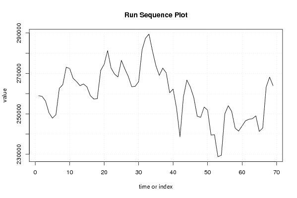
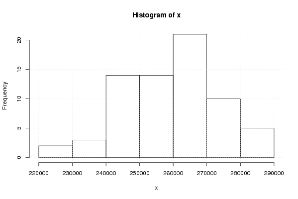
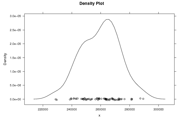
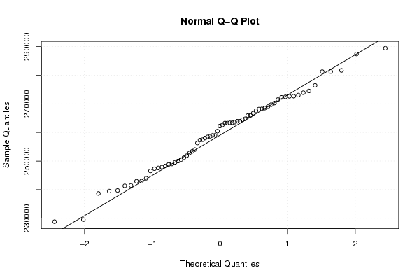
| Dataseries X: | |||||||||||||||||||||||||||||||||||||||||||||||||||||
258961 258647 256304 250498 247883 249552 262626 264416 273049 272441 267564 265952 263937 264765 263386 258985 257334 257477 271486 274488 281274 272674 269704 268227 276444 272247 268516 263406 263619 265905 281681 287413 289423 281242 273878 269022 272630 270287 260447 262248 252806 238663 258438 266719 263279 258064 248828 248284 253376 251846 239494 239709 228793 229521 249999 254016 251178 242936 241478 243985 246546 247323 247599 248985 241326 242967 263281 268145 263948 | |||||||||||||||||||||||||||||||||||||||||||||||||||||
Tables (Output of Computation) | |||||||||||||||||||||||||||||||||||||||||||||||||||||
| |||||||||||||||||||||||||||||||||||||||||||||||||||||
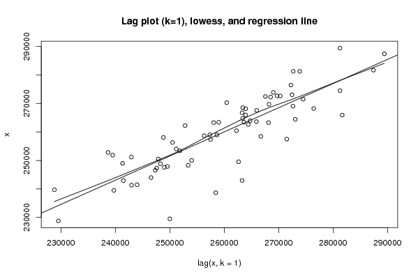
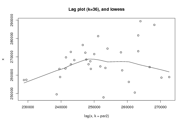
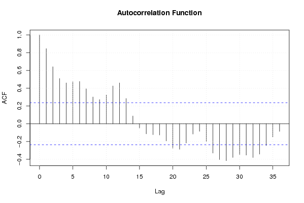
Figures (Output of Computation) | |||||||||||||||||||||||||||||||||||||||||||||||||||||
Input Parameters & R Code | |||||||||||||||||||||||||||||||||||||||||||||||||||||
| Parameters (Session): | |||||||||||||||||||||||||||||||||||||||||||||||||||||
| par1 = 0 ; par2 = 36 ; | |||||||||||||||||||||||||||||||||||||||||||||||||||||
| Parameters (R input): | |||||||||||||||||||||||||||||||||||||||||||||||||||||
| par1 = 0 ; par2 = 36 ; | |||||||||||||||||||||||||||||||||||||||||||||||||||||
| R code (references can be found in the software module): | |||||||||||||||||||||||||||||||||||||||||||||||||||||
par1 <- as.numeric(par1) | |||||||||||||||||||||||||||||||||||||||||||||||||||||