Free Statistics
of Irreproducible Research!
Description of Statistical Computation | |||||||||||||||||||||||||||||||||||||||||||||||||||||
|---|---|---|---|---|---|---|---|---|---|---|---|---|---|---|---|---|---|---|---|---|---|---|---|---|---|---|---|---|---|---|---|---|---|---|---|---|---|---|---|---|---|---|---|---|---|---|---|---|---|---|---|---|---|
| Author's title | |||||||||||||||||||||||||||||||||||||||||||||||||||||
| Author | *The author of this computation has been verified* | ||||||||||||||||||||||||||||||||||||||||||||||||||||
| R Software Module | rwasp_edauni.wasp | ||||||||||||||||||||||||||||||||||||||||||||||||||||
| Title produced by software | Univariate Explorative Data Analysis | ||||||||||||||||||||||||||||||||||||||||||||||||||||
| Date of computation | Mon, 19 Oct 2009 13:51:19 -0600 | ||||||||||||||||||||||||||||||||||||||||||||||||||||
| Cite this page as follows | Statistical Computations at FreeStatistics.org, Office for Research Development and Education, URL https://freestatistics.org/blog/index.php?v=date/2009/Oct/19/t1255981945tfahgw2sdfbdlad.htm/, Retrieved Mon, 29 Apr 2024 18:24:24 +0000 | ||||||||||||||||||||||||||||||||||||||||||||||||||||
| Statistical Computations at FreeStatistics.org, Office for Research Development and Education, URL https://freestatistics.org/blog/index.php?pk=48186, Retrieved Mon, 29 Apr 2024 18:24:24 +0000 | |||||||||||||||||||||||||||||||||||||||||||||||||||||
| QR Codes: | |||||||||||||||||||||||||||||||||||||||||||||||||||||
|
| |||||||||||||||||||||||||||||||||||||||||||||||||||||
| Original text written by user: | |||||||||||||||||||||||||||||||||||||||||||||||||||||
| IsPrivate? | No (this computation is public) | ||||||||||||||||||||||||||||||||||||||||||||||||||||
| User-defined keywords | |||||||||||||||||||||||||||||||||||||||||||||||||||||
| Estimated Impact | 100 | ||||||||||||||||||||||||||||||||||||||||||||||||||||
Tree of Dependent Computations | |||||||||||||||||||||||||||||||||||||||||||||||||||||
| Family? (F = Feedback message, R = changed R code, M = changed R Module, P = changed Parameters, D = changed Data) | |||||||||||||||||||||||||||||||||||||||||||||||||||||
| - [Univariate Explorative Data Analysis] [Workshop3 Part1 D...] [2009-10-19 09:05:14] [143cbdcaf7333bdd9926a1dde50d1082] - D [Univariate Explorative Data Analysis] [Workshop3 Part2 D...] [2009-10-19 19:48:55] [143cbdcaf7333bdd9926a1dde50d1082] - D [Univariate Explorative Data Analysis] [Workshop3 Part2 D...] [2009-10-19 19:51:19] [5ed0eef5d4509bbfdac0ae6d87f3b4bf] [Current] - D [Univariate Explorative Data Analysis] [Workshop3 Part2 D...] [2009-10-19 19:53:33] [143cbdcaf7333bdd9926a1dde50d1082] - RMPD [] [WS 3 gem verbetering] [1970-01-01 00:00:00] [830e13ac5e5ac1e5b21c6af0c149b21d] - RMPD [Harrell-Davis Quantiles] [WS 3 voorspelling...] [2009-10-23 12:36:30] [830e13ac5e5ac1e5b21c6af0c149b21d] | |||||||||||||||||||||||||||||||||||||||||||||||||||||
| Feedback Forum | |||||||||||||||||||||||||||||||||||||||||||||||||||||
Post a new message | |||||||||||||||||||||||||||||||||||||||||||||||||||||
Dataset | |||||||||||||||||||||||||||||||||||||||||||||||||||||
| Dataseries X: | |||||||||||||||||||||||||||||||||||||||||||||||||||||
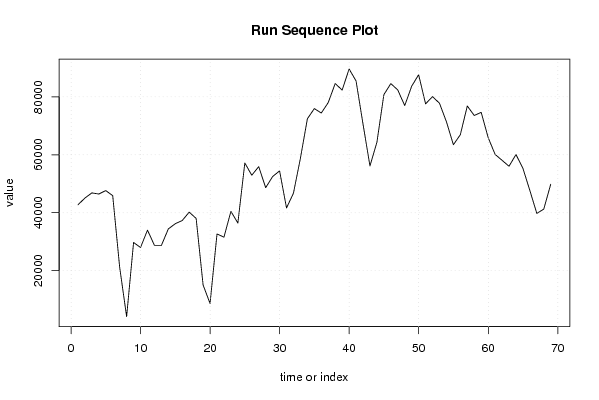
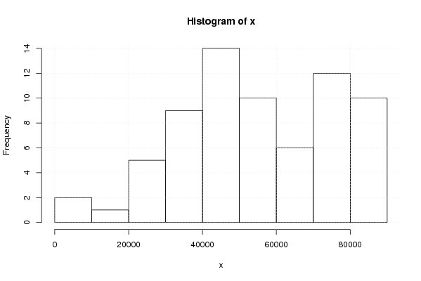
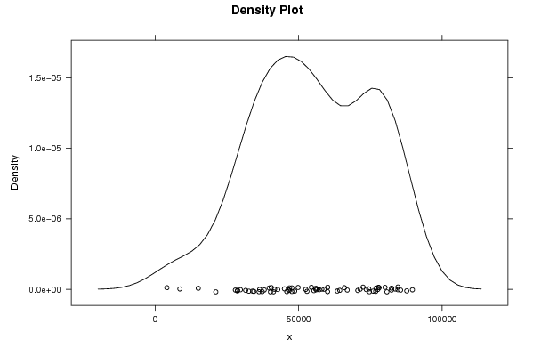
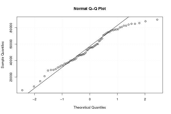
42727 45060 46839 46453 47646 45886 21150 4109 29725 27981 33989 28735 28694 34411 36202 37307 40192 38025 15040 8643 32650 31560 40459 36422 57167 52934 55906 48635 52477 54448 41633 46777 58843 72447 75956 74426 78049 84601 82341 89640 85504 70610 56138 64331 80763 84588 82384 76987 83675 87664 77580 80097 77792 71407 63469 66947 76848 73574 74651 65948 60134 58097 56036 60079 55321 47658 39749 41246 49822 | |||||||||||||||||||||||||||||||||||||||||||||||||||||
Tables (Output of Computation) | |||||||||||||||||||||||||||||||||||||||||||||||||||||
| |||||||||||||||||||||||||||||||||||||||||||||||||||||
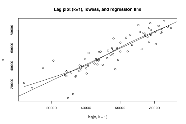
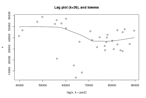
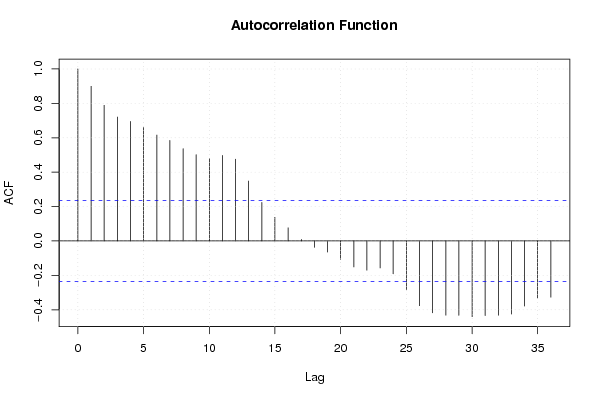
Figures (Output of Computation) | |||||||||||||||||||||||||||||||||||||||||||||||||||||
Input Parameters & R Code | |||||||||||||||||||||||||||||||||||||||||||||||||||||
| Parameters (Session): | |||||||||||||||||||||||||||||||||||||||||||||||||||||
| par1 = 0 ; par2 = 36 ; | |||||||||||||||||||||||||||||||||||||||||||||||||||||
| Parameters (R input): | |||||||||||||||||||||||||||||||||||||||||||||||||||||
| par1 = 0 ; par2 = 36 ; | |||||||||||||||||||||||||||||||||||||||||||||||||||||
| R code (references can be found in the software module): | |||||||||||||||||||||||||||||||||||||||||||||||||||||
par1 <- as.numeric(par1) | |||||||||||||||||||||||||||||||||||||||||||||||||||||