Repository of Reproducible Computations

Free Statistics

of Irreproducible Research!

Author's title

Author

*Unverified author*

R Software Module

rwasp_edauni.wasp

Title produced by software

Univariate Explorative Data Analysis

Date of computation

Tue, 20 Oct 2009 14:40:37 -0600

Cite this page as follows

Statistical Computations at FreeStatistics.org, Office for Research Development and Education, URL https://freestatistics.org/blog/index.php?v=date/2009/Oct/20/t1256071310unnry87lp73d9w1.htm/, Retrieved Mon, 06 May 2024 14:03:11 +0000

Statistical Computations at FreeStatistics.org, Office for Research Development and Education, URL https://freestatistics.org/blog/index.php?pk=49144, Retrieved Mon, 06 May 2024 14:03:11 +0000

QR Codes:

Paste this QR Code to cite your computation.

Original text written by user:

IsPrivate?

No (this computation is public)

User-defined keywords

Estimated Impact

136

Family? (F = Feedback message, R = changed R code, M = changed R Module, P = changed Parameters, D = changed Data)

-     [Univariate Data Series] [ws2:dollarkoers] [2009-10-07 14:57:42] [f14ab336a996fc02ebda5a25ed16c051]
- RMPD  [Univariate Explorative Data Analysis] [ws3- assumpties Y...] [2009-10-20 20:33:15] [74be16979710d4c4e7c6647856088456]
-    D      [Univariate Explorative Data Analysis] [ws3- assumpties e...] [2009-10-20 20:40:37] [d41d8cd98f00b204e9800998ecf8427e] [Current]

Feedback Forum

Post a new message

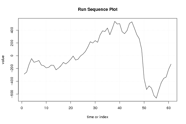
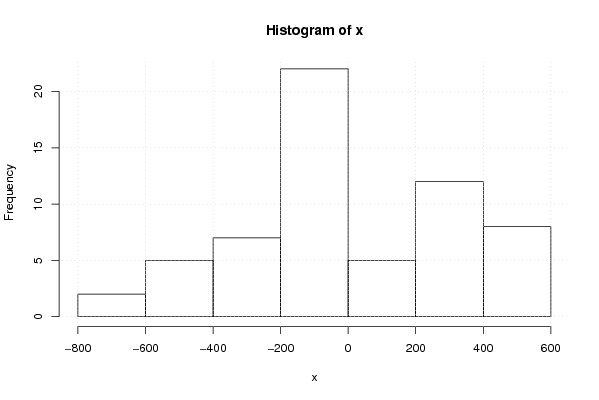
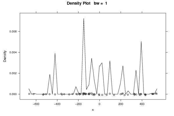
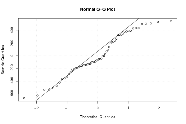
Dataseries X:

Download CSV

Histogram

Boxplots

-286,973012
-256,06057
-133,960046
-44,629232
-102,65134
-91,331518
-75,14251
-146,003404
-156,821368
-189,992875
-181,319712
-147,657316
-150,054704
-220,39006
-194,165718
-156,219808
-104,895184
-128,46523
-97,34634
-54,624922
-5,2
-67,3332
-54,041584
-3,562135
24,646787
66,828518
136,164303
218,985746
198,735584
236,20541
210,55319
325,73934
389,171254
379,764131
433,646168
328,953364
427,867952
537,944282
496,311876
502,70811
376,728968
345,632276
392,282738
505,96025
530,459354
433,516125
330,27941
266,471325
96,076717
-361,455014
-528,243472
-472,487842
-506,588638
-623,043445
-664,47535
-533,6223
-420,74035
-354,494224
-334,146784
-211,861504
-131,45629

Summary of computational transaction
Raw Input	view raw input (R code)
Raw Output	view raw output of R engine
Computing time	3 seconds
R Server	'Sir Ronald Aylmer Fisher' @ 193.190.124.24

\begin{tabular}{lllllllll}
\hline
Summary of computational transaction \tabularnewline
Raw Input & view raw input (R code)  \tabularnewline
Raw Output & view raw output of R engine  \tabularnewline
Computing time & 3 seconds \tabularnewline
R Server & 'Sir Ronald Aylmer Fisher' @ 193.190.124.24 \tabularnewline
\hline
\end{tabular}
%Source: https://freestatistics.org/blog/index.php?pk=49144&T=0

[TABLE]
[ROW][C]Summary of computational transaction[/C][/ROW]
[ROW][C]Raw Input[/C][C]view raw input (R code) [/C][/ROW]
[ROW][C]Raw Output[/C][C]view raw output of R engine [/C][/ROW]
[ROW][C]Computing time[/C][C]3 seconds[/C][/ROW]
[ROW][C]R Server[/C][C]'Sir Ronald Aylmer Fisher' @ 193.190.124.24[/C][/ROW]
[/TABLE]
Source: https://freestatistics.org/blog/index.php?pk=49144&T=0

Globally Unique Identifier (entire table): ba.freestatistics.org/blog/index.php?pk=49144&T=0

As an alternative you can also use a QR Code:

The GUIDs for individual cells are displayed in the table below:

Summary of computational transaction
Raw Input	view raw input (R code)
Raw Output	view raw output of R engine
Computing time	3 seconds
R Server	'Sir Ronald Aylmer Fisher' @ 193.190.124.24

Descriptive Statistics
# observations	61
minimum	-664.47535
Q1	-189.992875
median	-67.3332
mean	0.00288814754098185
Q3	325.73934
maximum	537.944282

\begin{tabular}{lllllllll}
\hline
Descriptive Statistics \tabularnewline
# observations & 61 \tabularnewline
minimum & -664.47535 \tabularnewline
Q1 & -189.992875 \tabularnewline
median & -67.3332 \tabularnewline
mean & 0.00288814754098185 \tabularnewline
Q3 & 325.73934 \tabularnewline
maximum & 537.944282 \tabularnewline
\hline
\end{tabular}
%Source: https://freestatistics.org/blog/index.php?pk=49144&T=1

[TABLE]
[ROW][C]Descriptive Statistics[/C][/ROW]
[ROW][C]# observations[/C][C]61[/C][/ROW]
[ROW][C]minimum[/C][C]-664.47535[/C][/ROW]
[ROW][C]Q1[/C][C]-189.992875[/C][/ROW]
[ROW][C]median[/C][C]-67.3332[/C][/ROW]
[ROW][C]mean[/C][C]0.00288814754098185[/C][/ROW]
[ROW][C]Q3[/C][C]325.73934[/C][/ROW]
[ROW][C]maximum[/C][C]537.944282[/C][/ROW]
[/TABLE]
Source: https://freestatistics.org/blog/index.php?pk=49144&T=1

Globally Unique Identifier (entire table): ba.freestatistics.org/blog/index.php?pk=49144&T=1

As an alternative you can also use a QR Code:

The GUIDs for individual cells are displayed in the table below:

Descriptive Statistics
# observations	61
minimum	-664.47535
Q1	-189.992875
median	-67.3332
mean	0.00288814754098185
Q3	325.73934
maximum	537.944282

Figure 1

PNG link

Postscript link

PDF link

Figure 2

PNG link

Postscript link

PDF link

Figure 3

PNG link

Postscript link

PDF link

Figure 4

PNG link

Postscript link

PDF link

Figure 5

PNG link

Postscript link

PDF link

Figure 6

PNG link

Postscript link

PDF link

Figure 7

PNG link

Postscript link

PDF link

Parameters (Session):

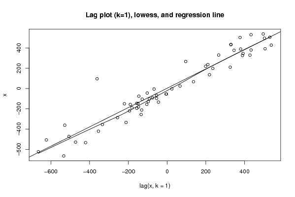
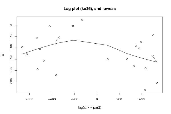
par1 = 1 ; par2 = 36 ;

Parameters (R input):

par1 = 1 ; par2 = 36 ;

R code (references can be found in the software module):

par1 <- as.numeric(par1)
par2 <- as.numeric(par2)
x <- as.ts(x)
library(lattice)
bitmap(file='pic1.png')
plot(x,type='l',main='Run Sequence Plot',xlab='time or index',ylab='value')
grid()
dev.off()
bitmap(file='pic2.png')
hist(x)
grid()
dev.off()
bitmap(file='pic3.png')
if (par1 > 0)
{
densityplot(~x,col='black',main=paste('Density Plot   bw = ',par1),bw=par1)
} else {
densityplot(~x,col='black',main='Density Plot')
}
dev.off()
bitmap(file='pic4.png')
qqnorm(x)
qqline(x)
grid()
dev.off()
if (par2 > 0)
{
bitmap(file='lagplot1.png')
dum <- cbind(lag(x,k=1),x)
dum
dum1 <- dum[2:length(x),]
dum1
z <- as.data.frame(dum1)
z
plot(z,main='Lag plot (k=1), lowess, and regression line')
lines(lowess(z))
abline(lm(z))
dev.off()
if (par2 > 1) {
bitmap(file='lagplotpar2.png')
dum <- cbind(lag(x,k=par2),x)
dum
dum1 <- dum[(par2+1):length(x),]
dum1
z <- as.data.frame(dum1)
z
mylagtitle <- 'Lag plot (k='
mylagtitle <- paste(mylagtitle,par2,sep='')
mylagtitle <- paste(mylagtitle,'), and lowess',sep='')
plot(z,main=mylagtitle)
lines(lowess(z))
dev.off()
}
bitmap(file='pic5.png')
acf(x,lag.max=par2,main='Autocorrelation Function')
grid()
dev.off()
}
summary(x)
load(file='createtable')
a<-table.start()
a<-table.row.start(a)
a<-table.element(a,'Descriptive Statistics',2,TRUE)
a<-table.row.end(a)
a<-table.row.start(a)
a<-table.element(a,'# observations',header=TRUE)
a<-table.element(a,length(x))
a<-table.row.end(a)
a<-table.row.start(a)
a<-table.element(a,'minimum',header=TRUE)
a<-table.element(a,min(x))
a<-table.row.end(a)
a<-table.row.start(a)
a<-table.element(a,'Q1',header=TRUE)
a<-table.element(a,quantile(x,0.25))
a<-table.row.end(a)
a<-table.row.start(a)
a<-table.element(a,'median',header=TRUE)
a<-table.element(a,median(x))
a<-table.row.end(a)
a<-table.row.start(a)
a<-table.element(a,'mean',header=TRUE)
a<-table.element(a,mean(x))
a<-table.row.end(a)
a<-table.row.start(a)
a<-table.element(a,'Q3',header=TRUE)
a<-table.element(a,quantile(x,0.75))
a<-table.row.end(a)
a<-table.row.start(a)
a<-table.element(a,'maximum',header=TRUE)
a<-table.element(a,max(x))
a<-table.row.end(a)
a<-table.end(a)
table.save(a,file='mytable.tab')

Free Statistics

Description of Statistical Computation

Tree of Dependent Computations

Dataset

Tables (Output of Computation)

Figures (Output of Computation)

Input Parameters & R Code