Free Statistics
of Irreproducible Research!
Description of Statistical Computation | |||||||||||||||||||||||||||||||||||||||||||||||||||||
|---|---|---|---|---|---|---|---|---|---|---|---|---|---|---|---|---|---|---|---|---|---|---|---|---|---|---|---|---|---|---|---|---|---|---|---|---|---|---|---|---|---|---|---|---|---|---|---|---|---|---|---|---|---|
| Author's title | |||||||||||||||||||||||||||||||||||||||||||||||||||||
| Author | *The author of this computation has been verified* | ||||||||||||||||||||||||||||||||||||||||||||||||||||
| R Software Module | rwasp_edauni.wasp | ||||||||||||||||||||||||||||||||||||||||||||||||||||
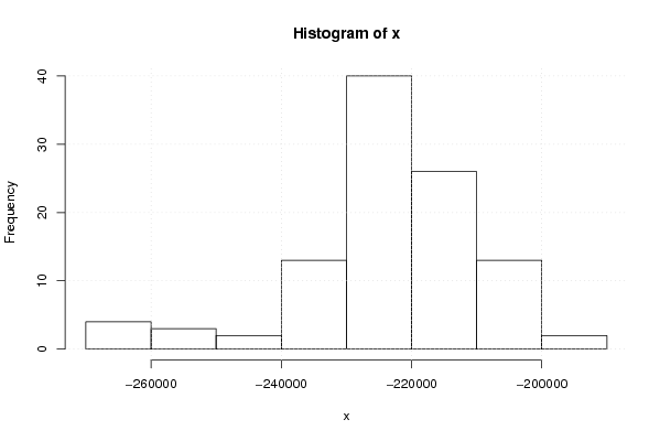
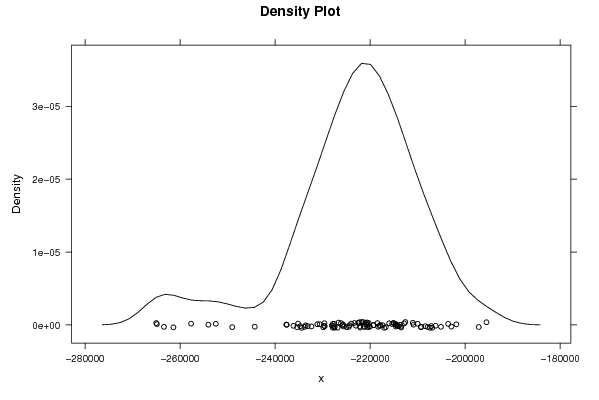
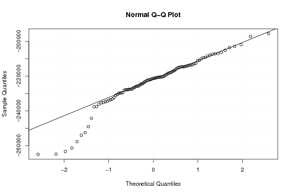
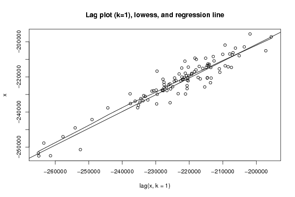
| Title produced by software | Univariate Explorative Data Analysis | ||||||||||||||||||||||||||||||||||||||||||||||||||||
| Date of computation | Wed, 21 Oct 2009 10:37:01 -0600 | ||||||||||||||||||||||||||||||||||||||||||||||||||||
| Cite this page as follows | Statistical Computations at FreeStatistics.org, Office for Research Development and Education, URL https://freestatistics.org/blog/index.php?v=date/2009/Oct/21/t1256143079jaw18ueg972obq1.htm/, Retrieved Thu, 02 May 2024 01:42:09 +0000 | ||||||||||||||||||||||||||||||||||||||||||||||||||||
| Statistical Computations at FreeStatistics.org, Office for Research Development and Education, URL https://freestatistics.org/blog/index.php?pk=49494, Retrieved Thu, 02 May 2024 01:42:09 +0000 | |||||||||||||||||||||||||||||||||||||||||||||||||||||
| QR Codes: | |||||||||||||||||||||||||||||||||||||||||||||||||||||
|
| |||||||||||||||||||||||||||||||||||||||||||||||||||||
| Original text written by user: | |||||||||||||||||||||||||||||||||||||||||||||||||||||
| IsPrivate? | No (this computation is public) | ||||||||||||||||||||||||||||||||||||||||||||||||||||
| User-defined keywords | |||||||||||||||||||||||||||||||||||||||||||||||||||||
| Estimated Impact | 108 | ||||||||||||||||||||||||||||||||||||||||||||||||||||
Tree of Dependent Computations | |||||||||||||||||||||||||||||||||||||||||||||||||||||
| Family? (F = Feedback message, R = changed R code, M = changed R Module, P = changed Parameters, D = changed Data) | |||||||||||||||||||||||||||||||||||||||||||||||||||||
| - [Bivariate Data Series] [Bivariate dataset] [2008-01-05 23:51:08] [74be16979710d4c4e7c6647856088456] F RMPD [Univariate Explorative Data Analysis] [Colombia Coffee] [2008-01-07 14:21:11] [74be16979710d4c4e7c6647856088456] F RMPD [Univariate Data Series] [] [2009-10-14 08:30:28] [74be16979710d4c4e7c6647856088456] - RMPD [Central Tendency] [] [2009-10-21 15:49:56] [9b30bff5dd5a100f8196daf92e735633] - RMPD [Univariate Explorative Data Analysis] [] [2009-10-21 16:37:01] [54e293c1fb7c46e2abc5c1dda68d8adb] [Current] | |||||||||||||||||||||||||||||||||||||||||||||||||||||
| Feedback Forum | |||||||||||||||||||||||||||||||||||||||||||||||||||||
Post a new message | |||||||||||||||||||||||||||||||||||||||||||||||||||||
Dataset | |||||||||||||||||||||||||||||||||||||||||||||||||||||
| Dataseries X: | |||||||||||||||||||||||||||||||||||||||||||||||||||||
-202894,96 -203571,96 -206213,96 -206930,96 -207906,96 -205083,96 -197142,96 -195508,96 -201852,96 -209312,96 -215093,96 -215980,96 -217984,96 -219246,96 -220070,96 -222194,96 -220307,96 -217341,96 -210856,96 -212591,96 -214402,96 -220278,96 -221472,96 -222057,96 -223961,96 -225764,96 -226832,96 -225576,96 -224942,96 -220644,96 -213456,96 -214605,96 -214919,96 -222231,96 -222503,96 -224459,96 -226122,96 -227499,96 -227843,96 -227748,96 -226647,96 -220635,96 -214625,96 -213560,96 -214212,96 -208381,96 -212828,96 -213997,96 -217012,96 -218448,96 -219267,96 -220821,96 -220445,96 -214579,96 -207404,96 -207109,96 -209989,96 -217876,96 -221171,96 -221792,96 -220593,96 -224365,96 -227494,96 -229848,96 -229550,96 -223301,96 -213658,96 -209264,96 -218305,96 -223008,96 -227531,96 -228069,96 -231113,96 -233119,96 -232344,96 -234408,96 -234697,96 -225703,96 -215371,96 -211016,96 -221290,96 -227837,96 -230619,96 -233573,96 -233781,96 -236138,96 -235159,96 -237548,96 -235372,96 -229719,96 -221110,96 -216697,96 -229614,96 -237643,96 -244281,96 -249010,96 -254037,96 -257677,96 -263391,96 -265012,96 -264884,96 -261393,96 -252471,96 | |||||||||||||||||||||||||||||||||||||||||||||||||||||
Tables (Output of Computation) | |||||||||||||||||||||||||||||||||||||||||||||||||||||
| |||||||||||||||||||||||||||||||||||||||||||||||||||||
Figures (Output of Computation) | |||||||||||||||||||||||||||||||||||||||||||||||||||||
Input Parameters & R Code | |||||||||||||||||||||||||||||||||||||||||||||||||||||
| Parameters (Session): | |||||||||||||||||||||||||||||||||||||||||||||||||||||
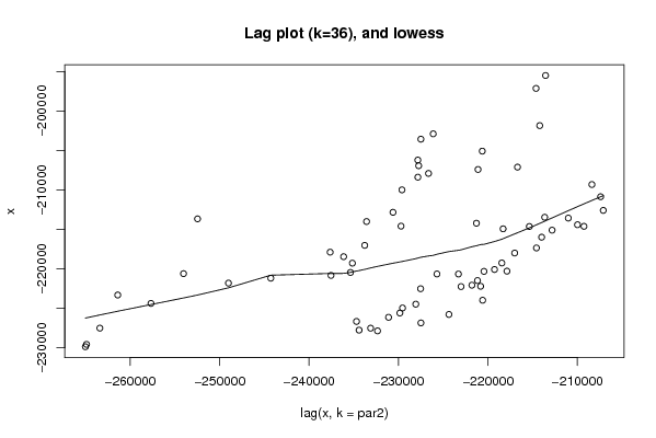
| par1 = 0 ; par2 = 36 ; | |||||||||||||||||||||||||||||||||||||||||||||||||||||
| Parameters (R input): | |||||||||||||||||||||||||||||||||||||||||||||||||||||
| par1 = 0 ; par2 = 36 ; | |||||||||||||||||||||||||||||||||||||||||||||||||||||
| R code (references can be found in the software module): | |||||||||||||||||||||||||||||||||||||||||||||||||||||
par1 <- as.numeric(par1) | |||||||||||||||||||||||||||||||||||||||||||||||||||||