Free Statistics
of Irreproducible Research!
Description of Statistical Computation | |||||||||||||||||||||||||||||||||||||||||||||||||||||
|---|---|---|---|---|---|---|---|---|---|---|---|---|---|---|---|---|---|---|---|---|---|---|---|---|---|---|---|---|---|---|---|---|---|---|---|---|---|---|---|---|---|---|---|---|---|---|---|---|---|---|---|---|---|
| Author's title | |||||||||||||||||||||||||||||||||||||||||||||||||||||
| Author | *The author of this computation has been verified* | ||||||||||||||||||||||||||||||||||||||||||||||||||||
| R Software Module | rwasp_edauni.wasp | ||||||||||||||||||||||||||||||||||||||||||||||||||||
| Title produced by software | Univariate Explorative Data Analysis | ||||||||||||||||||||||||||||||||||||||||||||||||||||
| Date of computation | Wed, 21 Oct 2009 10:45:15 -0600 | ||||||||||||||||||||||||||||||||||||||||||||||||||||
| Cite this page as follows | Statistical Computations at FreeStatistics.org, Office for Research Development and Education, URL https://freestatistics.org/blog/index.php?v=date/2009/Oct/21/t12561435666wsgyyz9owggq19.htm/, Retrieved Thu, 02 May 2024 07:34:57 +0000 | ||||||||||||||||||||||||||||||||||||||||||||||||||||
| Statistical Computations at FreeStatistics.org, Office for Research Development and Education, URL https://freestatistics.org/blog/index.php?pk=49500, Retrieved Thu, 02 May 2024 07:34:57 +0000 | |||||||||||||||||||||||||||||||||||||||||||||||||||||
| QR Codes: | |||||||||||||||||||||||||||||||||||||||||||||||||||||
|
| |||||||||||||||||||||||||||||||||||||||||||||||||||||
| Original text written by user: | |||||||||||||||||||||||||||||||||||||||||||||||||||||
| IsPrivate? | No (this computation is public) | ||||||||||||||||||||||||||||||||||||||||||||||||||||
| User-defined keywords | |||||||||||||||||||||||||||||||||||||||||||||||||||||
| Estimated Impact | 57 | ||||||||||||||||||||||||||||||||||||||||||||||||||||
Tree of Dependent Computations | |||||||||||||||||||||||||||||||||||||||||||||||||||||
| Family? (F = Feedback message, R = changed R code, M = changed R Module, P = changed Parameters, D = changed Data) | |||||||||||||||||||||||||||||||||||||||||||||||||||||
| - [Bivariate Data Series] [Bivariate dataset] [2008-01-05 23:51:08] [74be16979710d4c4e7c6647856088456] F RMPD [Univariate Explorative Data Analysis] [Colombia Coffee] [2008-01-07 14:21:11] [74be16979710d4c4e7c6647856088456] F RMPD [Univariate Data Series] [] [2009-10-14 08:30:28] [74be16979710d4c4e7c6647856088456] - RMPD [Central Tendency] [] [2009-10-21 15:49:56] [9b30bff5dd5a100f8196daf92e735633] - RMPD [Univariate Explorative Data Analysis] [] [2009-10-21 16:45:15] [54e293c1fb7c46e2abc5c1dda68d8adb] [Current] | |||||||||||||||||||||||||||||||||||||||||||||||||||||
| Feedback Forum | |||||||||||||||||||||||||||||||||||||||||||||||||||||
Post a new message | |||||||||||||||||||||||||||||||||||||||||||||||||||||
Dataset | |||||||||||||||||||||||||||||||||||||||||||||||||||||
| Dataseries X: | |||||||||||||||||||||||||||||||||||||||||||||||||||||
-253620,7163 -253620,7159 -253620,7233 -253620,7243 -253620,7258 -253620,7064 -253620,6958 -253620,7026 -253620,7355 -253620,7667 -253620,7818 -253620,7863 -253620,7982 -253620,8038 -253620,8064 -253620,8138 -253620,8019 -253620,787 -253620,7796 -253620,7905 -253620,7979 -253620,8226 -253620,8252 -253620,8287 -253620,8388 -253620,8461 -253620,8491 -253620,8434 -253620,8385 -253620,8209 -253620,8082 -253620,8157 -253620,8165 -253620,8425 -253620,8394 -253620,849 -253620,8572 -253620,8623 -253620,8626 -253620,8601 -253620,8542 -253620,8306 -253620,8194 -253620,8196 -253620,8225 -253620,8002 -253620,8126 -253620,8174 -253620,8279 -253620,8331 -253620,8351 -253620,8386 -253620,8358 -253620,8127 -253620,7991 -253620,8003 -253620,8107 -253620,836 -253620,8447 -253620,8474 -253620,8421 -253620,8557 -253620,8656 -253620,8736 -253620,8723 -253620,8482 -253620,8221 -253620,8074 -253620,8392 -253620,8501 -253620,8633 -253620,8639 -253620,8763 -253620,8824 -253620,8766 -253620,8842 -253620,8831 -253620,8414 -253620,8121 -253620,7968 -253620,833 -253620,8571 -253620,8655 -253620,8789 -253620,8802 -253620,8887 -253620,8821 -253620,8922 -253620,8791 -253620,8546 -253620,8289 -253620,8113 -253620,8628 -253620,8948 -253620,9221 -253620,942 -253620,9616 -253620,9751 -253620,9958 -253621,0016 -253621,0021 -253620,9886 -253620,9561 | |||||||||||||||||||||||||||||||||||||||||||||||||||||
Tables (Output of Computation) | |||||||||||||||||||||||||||||||||||||||||||||||||||||
| |||||||||||||||||||||||||||||||||||||||||||||||||||||
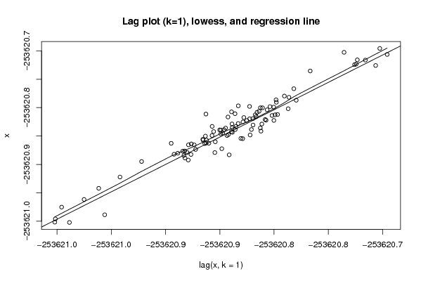
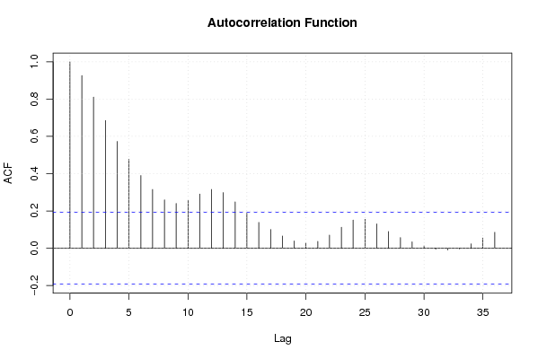
Figures (Output of Computation) | |||||||||||||||||||||||||||||||||||||||||||||||||||||
Input Parameters & R Code | |||||||||||||||||||||||||||||||||||||||||||||||||||||
| Parameters (Session): | |||||||||||||||||||||||||||||||||||||||||||||||||||||
| par1 = 0 ; par2 = 36 ; | |||||||||||||||||||||||||||||||||||||||||||||||||||||
| Parameters (R input): | |||||||||||||||||||||||||||||||||||||||||||||||||||||
| par1 = 0 ; par2 = 36 ; | |||||||||||||||||||||||||||||||||||||||||||||||||||||
| R code (references can be found in the software module): | |||||||||||||||||||||||||||||||||||||||||||||||||||||
par1 <- as.numeric(par1) | |||||||||||||||||||||||||||||||||||||||||||||||||||||