Repository of Reproducible Computations

Free Statistics

of Irreproducible Research!

Author's title

Author

*The author of this computation has been verified*

R Software Module

rwasp_edauni.wasp

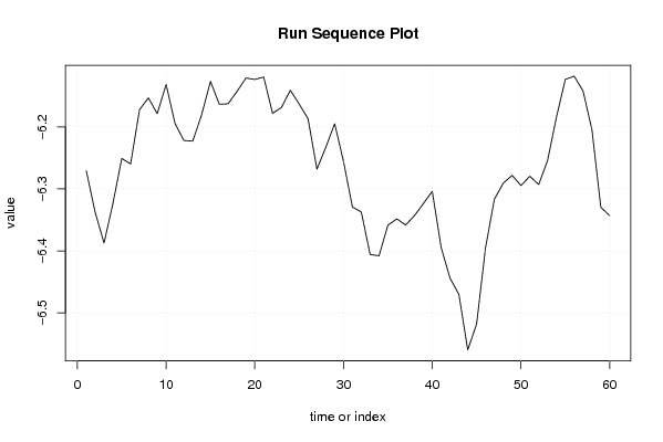
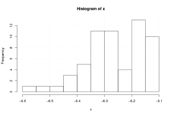
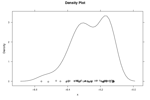
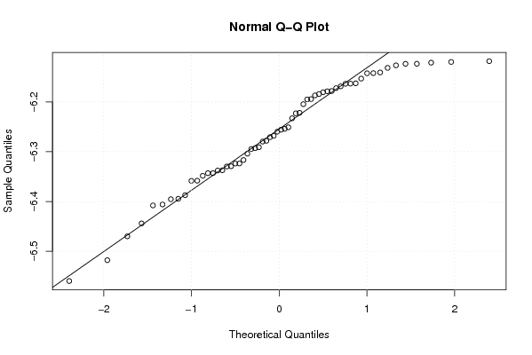
Title produced by software

Univariate Explorative Data Analysis

Date of computation

Sun, 25 Oct 2009 06:54:24 -0600

Cite this page as follows

Statistical Computations at FreeStatistics.org, Office for Research Development and Education, URL https://freestatistics.org/blog/index.php?v=date/2009/Oct/25/t1256475350zqfbflyfx7b4jgi.htm/, Retrieved Mon, 29 Apr 2024 09:01:46 +0000

Statistical Computations at FreeStatistics.org, Office for Research Development and Education, URL https://freestatistics.org/blog/index.php?pk=50306, Retrieved Mon, 29 Apr 2024 09:01:46 +0000

QR Codes:

Paste this QR Code to cite your computation.

Original text written by user:

IsPrivate?

No (this computation is public)

User-defined keywords

Estimated Impact

187

Family? (F = Feedback message, R = changed R code, M = changed R Module, P = changed Parameters, D = changed Data)

-       [Univariate Explorative Data Analysis] [SHW WS4 - Part 2 ...] [2009-10-25 12:54:24] [b7e46d23597387652ca7420fdeb9acca] [Current]

Feedback Forum

Post a new message

Dataseries X:

Download CSV

Histogram

Boxplots

-6,270809992
-6,337676883
-6,387313859
-6,323720438
-6,250903546
-6,259734647
-6,172173032
-6,153124912
-6,178580053
-6,131570874
-6,194287577
-6,221873567
-6,222920674
-6,180458492
-6,126462066
-6,163542449
-6,162530678
-6,142439097
-6,121115029
-6,123391871
-6,119609187
-6,178036747
-6,168624035
-6,140792082
-6,163150655
-6,186839915
-6,26804001
-6,232887748
-6,194876105
-6,255870593
-6,329221174
-6,337237947
-6,405952789
-6,40790481
-6,358536668
-6,348366148
-6,35823036
-6,343013121
-6,323667283
-6,303936625
-6,394566479
-6,444014089
-6,470017866
-6,559767409
-6,517893294
-6,395374224
-6,316695279
-6,290907138
-6,278070133
-6,294615446
-6,279596732
-6,292930598
-6,254019229
-6,184124411
-6,123315559
-6,118130279
-6,142098661
-6,204419549
-6,329659781
-6,343122035

Summary of computational transaction
Raw Input	view raw input (R code)
Raw Output	view raw output of R engine
Computing time	4 seconds
R Server	'Sir Ronald Aylmer Fisher' @ 193.190.124.24

\begin{tabular}{lllllllll}
\hline
Summary of computational transaction \tabularnewline
Raw Input & view raw input (R code)  \tabularnewline
Raw Output & view raw output of R engine  \tabularnewline
Computing time & 4 seconds \tabularnewline
R Server & 'Sir Ronald Aylmer Fisher' @ 193.190.124.24 \tabularnewline
\hline
\end{tabular}
%Source: https://freestatistics.org/blog/index.php?pk=50306&T=0

[TABLE]
[ROW][C]Summary of computational transaction[/C][/ROW]
[ROW][C]Raw Input[/C][C]view raw input (R code) [/C][/ROW]
[ROW][C]Raw Output[/C][C]view raw output of R engine [/C][/ROW]
[ROW][C]Computing time[/C][C]4 seconds[/C][/ROW]
[ROW][C]R Server[/C][C]'Sir Ronald Aylmer Fisher' @ 193.190.124.24[/C][/ROW]
[/TABLE]
Source: https://freestatistics.org/blog/index.php?pk=50306&T=0

Globally Unique Identifier (entire table): ba.freestatistics.org/blog/index.php?pk=50306&T=0

As an alternative you can also use a QR Code:

The GUIDs for individual cells are displayed in the table below:

Summary of computational transaction
Raw Input	view raw input (R code)
Raw Output	view raw output of R engine
Computing time	4 seconds
R Server	'Sir Ronald Aylmer Fisher' @ 193.190.124.24

Descriptive Statistics
# observations	60
minimum	-6.559767409
Q1	-6.337347681
median	-6.25780262
mean	-6.26304603215
Q3	-6.17128578275
maximum	-6.118130279

\begin{tabular}{lllllllll}
\hline
Descriptive Statistics \tabularnewline
# observations & 60 \tabularnewline
minimum & -6.559767409 \tabularnewline
Q1 & -6.337347681 \tabularnewline
median & -6.25780262 \tabularnewline
mean & -6.26304603215 \tabularnewline
Q3 & -6.17128578275 \tabularnewline
maximum & -6.118130279 \tabularnewline
\hline
\end{tabular}
%Source: https://freestatistics.org/blog/index.php?pk=50306&T=1

[TABLE]
[ROW][C]Descriptive Statistics[/C][/ROW]
[ROW][C]# observations[/C][C]60[/C][/ROW]
[ROW][C]minimum[/C][C]-6.559767409[/C][/ROW]
[ROW][C]Q1[/C][C]-6.337347681[/C][/ROW]
[ROW][C]median[/C][C]-6.25780262[/C][/ROW]
[ROW][C]mean[/C][C]-6.26304603215[/C][/ROW]
[ROW][C]Q3[/C][C]-6.17128578275[/C][/ROW]
[ROW][C]maximum[/C][C]-6.118130279[/C][/ROW]
[/TABLE]
Source: https://freestatistics.org/blog/index.php?pk=50306&T=1

Globally Unique Identifier (entire table): ba.freestatistics.org/blog/index.php?pk=50306&T=1

As an alternative you can also use a QR Code:

The GUIDs for individual cells are displayed in the table below:

Descriptive Statistics
# observations	60
minimum	-6.559767409
Q1	-6.337347681
median	-6.25780262
mean	-6.26304603215
Q3	-6.17128578275
maximum	-6.118130279

Figure 1

PNG link

Postscript link

PDF link

Figure 2

PNG link

Postscript link

PDF link

Figure 3

PNG link

Postscript link

PDF link

Figure 4

PNG link

Postscript link

PDF link

Figure 5

PNG link

Postscript link

PDF link

Figure 6

PNG link

Postscript link

PDF link

Figure 7

PNG link

Postscript link

PDF link

Parameters (Session):

par1 = 0 ; par2 = 36 ;

Parameters (R input):

par1 = 0 ; par2 = 36 ;

R code (references can be found in the software module):

par1 <- as.numeric(par1)
par2 <- as.numeric(par2)
x <- as.ts(x)
library(lattice)
bitmap(file='pic1.png')
plot(x,type='l',main='Run Sequence Plot',xlab='time or index',ylab='value')
grid()
dev.off()
bitmap(file='pic2.png')
hist(x)
grid()
dev.off()
bitmap(file='pic3.png')
if (par1 > 0)
{
densityplot(~x,col='black',main=paste('Density Plot   bw = ',par1),bw=par1)
} else {
densityplot(~x,col='black',main='Density Plot')
}
dev.off()
bitmap(file='pic4.png')
qqnorm(x)
qqline(x)
grid()
dev.off()
if (par2 > 0)
{
bitmap(file='lagplot1.png')
dum <- cbind(lag(x,k=1),x)
dum
dum1 <- dum[2:length(x),]
dum1
z <- as.data.frame(dum1)
z
plot(z,main='Lag plot (k=1), lowess, and regression line')
lines(lowess(z))
abline(lm(z))
dev.off()
if (par2 > 1) {
bitmap(file='lagplotpar2.png')
dum <- cbind(lag(x,k=par2),x)
dum
dum1 <- dum[(par2+1):length(x),]
dum1
z <- as.data.frame(dum1)
z
mylagtitle <- 'Lag plot (k='
mylagtitle <- paste(mylagtitle,par2,sep='')
mylagtitle <- paste(mylagtitle,'), and lowess',sep='')
plot(z,main=mylagtitle)
lines(lowess(z))
dev.off()
}
bitmap(file='pic5.png')
acf(x,lag.max=par2,main='Autocorrelation Function')
grid()
dev.off()
}
summary(x)
load(file='createtable')
a<-table.start()
a<-table.row.start(a)
a<-table.element(a,'Descriptive Statistics',2,TRUE)
a<-table.row.end(a)
a<-table.row.start(a)
a<-table.element(a,'# observations',header=TRUE)
a<-table.element(a,length(x))
a<-table.row.end(a)
a<-table.row.start(a)
a<-table.element(a,'minimum',header=TRUE)
a<-table.element(a,min(x))
a<-table.row.end(a)
a<-table.row.start(a)
a<-table.element(a,'Q1',header=TRUE)
a<-table.element(a,quantile(x,0.25))
a<-table.row.end(a)
a<-table.row.start(a)
a<-table.element(a,'median',header=TRUE)
a<-table.element(a,median(x))
a<-table.row.end(a)
a<-table.row.start(a)
a<-table.element(a,'mean',header=TRUE)
a<-table.element(a,mean(x))
a<-table.row.end(a)
a<-table.row.start(a)
a<-table.element(a,'Q3',header=TRUE)
a<-table.element(a,quantile(x,0.75))
a<-table.row.end(a)
a<-table.row.start(a)
a<-table.element(a,'maximum',header=TRUE)
a<-table.element(a,max(x))
a<-table.row.end(a)
a<-table.end(a)
table.save(a,file='mytable.tab')

Free Statistics

Description of Statistical Computation

Tree of Dependent Computations

Dataset

Tables (Output of Computation)

Figures (Output of Computation)

Input Parameters & R Code