Free Statistics
of Irreproducible Research!
Description of Statistical Computation | |||||||||||||||||||||||||||||||||||||||||||||||||||||
|---|---|---|---|---|---|---|---|---|---|---|---|---|---|---|---|---|---|---|---|---|---|---|---|---|---|---|---|---|---|---|---|---|---|---|---|---|---|---|---|---|---|---|---|---|---|---|---|---|---|---|---|---|---|
| Author's title | |||||||||||||||||||||||||||||||||||||||||||||||||||||
| Author | *The author of this computation has been verified* | ||||||||||||||||||||||||||||||||||||||||||||||||||||
| R Software Module | rwasp_edauni.wasp | ||||||||||||||||||||||||||||||||||||||||||||||||||||
| Title produced by software | Univariate Explorative Data Analysis | ||||||||||||||||||||||||||||||||||||||||||||||||||||
| Date of computation | Sun, 25 Oct 2009 14:43:54 -0600 | ||||||||||||||||||||||||||||||||||||||||||||||||||||
| Cite this page as follows | Statistical Computations at FreeStatistics.org, Office for Research Development and Education, URL https://freestatistics.org/blog/index.php?v=date/2009/Oct/25/t12565034972bkjbk4swmxyfu0.htm/, Retrieved Mon, 29 Apr 2024 14:38:33 +0000 | ||||||||||||||||||||||||||||||||||||||||||||||||||||
| Statistical Computations at FreeStatistics.org, Office for Research Development and Education, URL https://freestatistics.org/blog/index.php?pk=50395, Retrieved Mon, 29 Apr 2024 14:38:33 +0000 | |||||||||||||||||||||||||||||||||||||||||||||||||||||
| QR Codes: | |||||||||||||||||||||||||||||||||||||||||||||||||||||
|
| |||||||||||||||||||||||||||||||||||||||||||||||||||||
| Original text written by user: | |||||||||||||||||||||||||||||||||||||||||||||||||||||
| IsPrivate? | No (this computation is public) | ||||||||||||||||||||||||||||||||||||||||||||||||||||
| User-defined keywords | |||||||||||||||||||||||||||||||||||||||||||||||||||||
| Estimated Impact | 145 | ||||||||||||||||||||||||||||||||||||||||||||||||||||
Tree of Dependent Computations | |||||||||||||||||||||||||||||||||||||||||||||||||||||
| Family? (F = Feedback message, R = changed R code, M = changed R Module, P = changed Parameters, D = changed Data) | |||||||||||||||||||||||||||||||||||||||||||||||||||||
| - [Bivariate Data Series] [Bivariate dataset] [2008-01-05 23:51:08] [74be16979710d4c4e7c6647856088456] F RMPD [Univariate Explorative Data Analysis] [Colombia Coffee] [2008-01-07 14:21:11] [74be16979710d4c4e7c6647856088456] F RMPD [Univariate Data Series] [] [2009-10-14 08:30:28] [74be16979710d4c4e7c6647856088456] - RMPD [Harrell-Davis Quantiles] [workshop 3] [2009-10-19 09:21:19] [3d8acb8ffdb376c5fec19e610f8198c2] - RMP [Univariate Explorative Data Analysis] [] [2009-10-25 20:43:54] [6c94b261890ba36343a04d1029691995] [Current] | |||||||||||||||||||||||||||||||||||||||||||||||||||||
| Feedback Forum | |||||||||||||||||||||||||||||||||||||||||||||||||||||
Post a new message | |||||||||||||||||||||||||||||||||||||||||||||||||||||
Dataset | |||||||||||||||||||||||||||||||||||||||||||||||||||||
| Dataseries X: | |||||||||||||||||||||||||||||||||||||||||||||||||||||
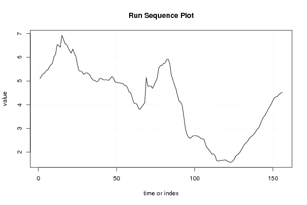
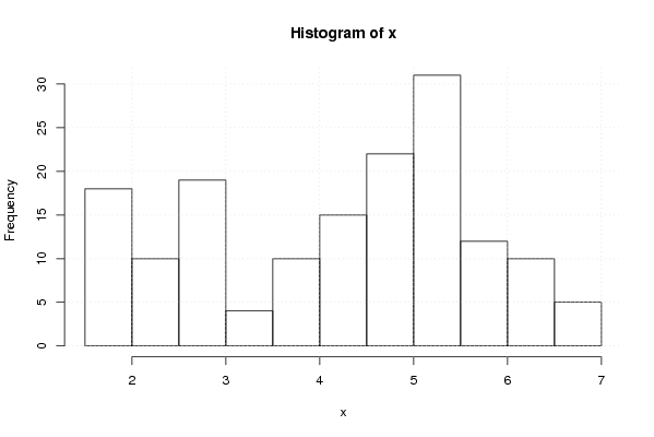
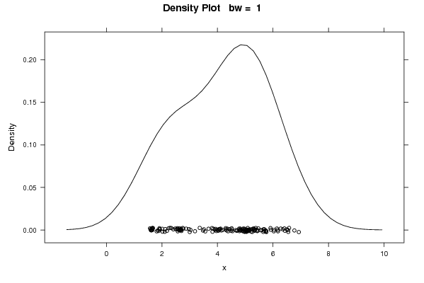
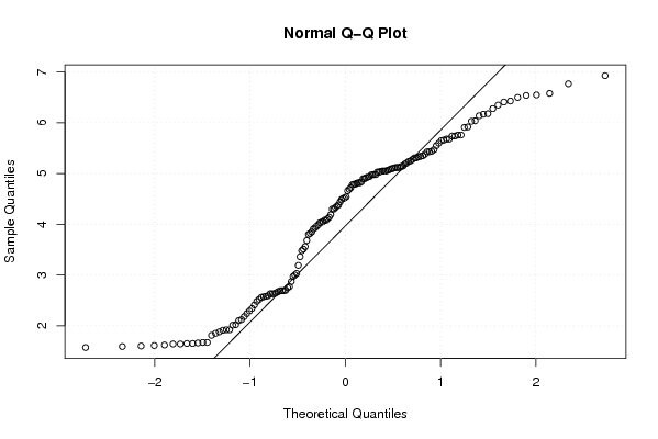
5.10 5.21 5.31 5.34 5.44 5.47 5.60 5.68 5.76 6.03 6.14 6.54 6.50 6.43 6.93 6.77 6.58 6.55 6.41 6.28 6.18 6.35 6.17 6.04 5.68 5.43 5.43 5.38 5.28 5.33 5.35 5.31 5.24 5.12 5.04 5.03 4.98 4.98 5.09 5.12 5.07 5.05 5.05 5.05 5.03 5.11 5.19 5.14 4.97 4.94 4.93 4.92 4.90 4.90 4.82 4.81 4.72 4.54 4.51 4.30 4.08 4.05 4.03 3.85 3.80 3.91 3.99 4.08 5.15 4.78 4.79 4.79 4.69 4.82 4.98 5.12 5.55 5.65 5.66 5.74 5.76 5.91 5.92 5.74 5.25 5.06 4.84 4.66 4.38 4.14 4.11 3.96 3.51 3.00 2.75 2.63 2.58 2.63 2.69 2.69 2.69 2.67 2.63 2.57 2.56 2.52 2.29 2.18 2.10 2.02 1.91 1.92 1.85 1.64 1.62 1.64 1.65 1.65 1.67 1.66 1.61 1.59 1.57 1.60 1.67 1.81 1.88 1.92 2.01 2.12 2.24 2.34 2.41 2.48 2.59 2.65 2.70 2.77 2.87 2.97 3.03 3.19 3.36 3.48 3.56 3.68 3.82 3.93 4.04 4.19 4.30 4.33 4.36 4.44 4.49 4.52 | |||||||||||||||||||||||||||||||||||||||||||||||||||||
Tables (Output of Computation) | |||||||||||||||||||||||||||||||||||||||||||||||||||||
| |||||||||||||||||||||||||||||||||||||||||||||||||||||
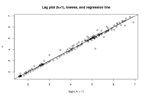
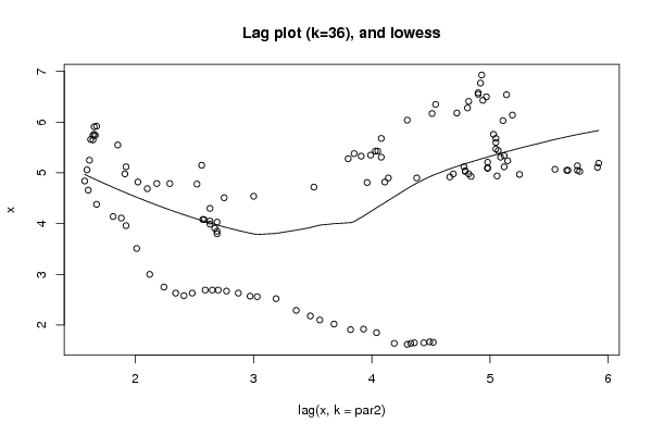
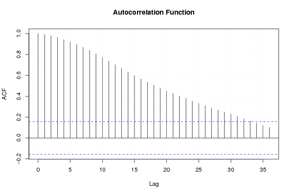
Figures (Output of Computation) | |||||||||||||||||||||||||||||||||||||||||||||||||||||
Input Parameters & R Code | |||||||||||||||||||||||||||||||||||||||||||||||||||||
| Parameters (Session): | |||||||||||||||||||||||||||||||||||||||||||||||||||||
| par1 = 1 ; par2 = 36 ; | |||||||||||||||||||||||||||||||||||||||||||||||||||||
| Parameters (R input): | |||||||||||||||||||||||||||||||||||||||||||||||||||||
| par1 = 1 ; par2 = 36 ; | |||||||||||||||||||||||||||||||||||||||||||||||||||||
| R code (references can be found in the software module): | |||||||||||||||||||||||||||||||||||||||||||||||||||||
par1 <- as.numeric(par1) | |||||||||||||||||||||||||||||||||||||||||||||||||||||