Repository of Reproducible Computations

Free Statistics

of Irreproducible Research!

Author's title

Author

*The author of this computation has been verified*

R Software Module

rwasp_edauni.wasp

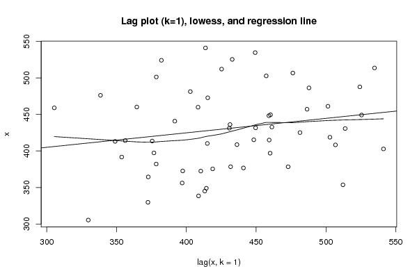
Title produced by software

Univariate Explorative Data Analysis

Date of computation

Mon, 26 Oct 2009 15:00:31 -0600

Cite this page as follows

Statistical Computations at FreeStatistics.org, Office for Research Development and Education, URL https://freestatistics.org/blog/index.php?v=date/2009/Oct/26/t12565910141zpjrcqfmp50r8l.htm/, Retrieved Thu, 02 May 2024 15:14:34 +0000

Statistical Computations at FreeStatistics.org, Office for Research Development and Education, URL https://freestatistics.org/blog/index.php?pk=50755, Retrieved Thu, 02 May 2024 15:14:34 +0000

QR Codes:

Paste this QR Code to cite your computation.

Original text written by user:

IsPrivate?

No (this computation is public)

User-defined keywords

Estimated Impact

163

Family? (F = Feedback message, R = changed R code, M = changed R Module, P = changed Parameters, D = changed Data)

-     [Bivariate Data Series] [Bivariate dataset] [2008-01-05 23:51:08] [74be16979710d4c4e7c6647856088456]
F RMPD  [Univariate Explorative Data Analysis] [Colombia Coffee] [2008-01-07 14:21:11] [74be16979710d4c4e7c6647856088456]
F RMPD    [Univariate Data Series] [] [2009-10-14 08:30:28] [74be16979710d4c4e7c6647856088456]
- RMPD      [Univariate Explorative Data Analysis] [SHWS] [2009-10-19 19:25:48] [a66d3a79ef9e5308cd94a469bc5ca464]
-    D          [Univariate Explorative Data Analysis] [Assumpties Yt/Xt] [2009-10-26 21:00:31] [f1100e00818182135823a11ccbd0f3b9] [Current]

Feedback Forum

Post a new message

Dataseries X:

Download CSV

Histogram

Boxplots

345,0561798
413,1707317
348,9473684
414,2857143
356,1728395
396,9879518
460
408,3544304
506,7948718
476,25
338,4705882
408,7209302
436,2352941
431,25
430,7692308
513,75
534,7560976
449,2771084
525,4878049
432,8395062
461,25
501,4102564
378,4615385
431,6883117
449,6052632
460,2631579
364,4736842
372,6923077
397,375
376,75
440,8860759
391,6883117
353,6486486
512,173913
425,2238806
481,3846154
402,8125
541,1940299
413,6764706
375,5072464
418,8405797
502,8358209
457,1875
486,4516129
487,7966102
524,2622951
382,0895522
378,3823529
472,8787879
415,3125
448,28125
459,1044776
305,3521127
329,7183099
372,4637681
410,3125
415
459,3333333

Summary of computational transaction
Raw Input	view raw input (R code)
Raw Output	view raw output of R engine
Computing time	5 seconds
R Server	'Gwilym Jenkins' @ 72.249.127.135

\begin{tabular}{lllllllll}
\hline
Summary of computational transaction \tabularnewline
Raw Input & view raw input (R code)  \tabularnewline
Raw Output & view raw output of R engine  \tabularnewline
Computing time & 5 seconds \tabularnewline
R Server & 'Gwilym Jenkins' @ 72.249.127.135 \tabularnewline
\hline
\end{tabular}
%Source: https://freestatistics.org/blog/index.php?pk=50755&T=0

[TABLE]
[ROW][C]Summary of computational transaction[/C][/ROW]
[ROW][C]Raw Input[/C][C]view raw input (R code) [/C][/ROW]
[ROW][C]Raw Output[/C][C]view raw output of R engine [/C][/ROW]
[ROW][C]Computing time[/C][C]5 seconds[/C][/ROW]
[ROW][C]R Server[/C][C]'Gwilym Jenkins' @ 72.249.127.135[/C][/ROW]
[/TABLE]
Source: https://freestatistics.org/blog/index.php?pk=50755&T=0

Globally Unique Identifier (entire table): ba.freestatistics.org/blog/index.php?pk=50755&T=0

As an alternative you can also use a QR Code:

The GUIDs for individual cells are displayed in the table below:

Summary of computational transaction
Raw Input	view raw input (R code)
Raw Output	view raw output of R engine
Computing time	5 seconds
R Server	'Gwilym Jenkins' @ 72.249.127.135

Descriptive Statistics
# observations	58
minimum	305.3521127
Q1	384.489242075
median	427.9965557
mean	429.057676262069
Q3	461.003289475
maximum	541.1940299

\begin{tabular}{lllllllll}
\hline
Descriptive Statistics \tabularnewline
# observations & 58 \tabularnewline
minimum & 305.3521127 \tabularnewline
Q1 & 384.489242075 \tabularnewline
median & 427.9965557 \tabularnewline
mean & 429.057676262069 \tabularnewline
Q3 & 461.003289475 \tabularnewline
maximum & 541.1940299 \tabularnewline
\hline
\end{tabular}
%Source: https://freestatistics.org/blog/index.php?pk=50755&T=1

[TABLE]
[ROW][C]Descriptive Statistics[/C][/ROW]
[ROW][C]# observations[/C][C]58[/C][/ROW]
[ROW][C]minimum[/C][C]305.3521127[/C][/ROW]
[ROW][C]Q1[/C][C]384.489242075[/C][/ROW]
[ROW][C]median[/C][C]427.9965557[/C][/ROW]
[ROW][C]mean[/C][C]429.057676262069[/C][/ROW]
[ROW][C]Q3[/C][C]461.003289475[/C][/ROW]
[ROW][C]maximum[/C][C]541.1940299[/C][/ROW]
[/TABLE]
Source: https://freestatistics.org/blog/index.php?pk=50755&T=1

Globally Unique Identifier (entire table): ba.freestatistics.org/blog/index.php?pk=50755&T=1

As an alternative you can also use a QR Code:

The GUIDs for individual cells are displayed in the table below:

Descriptive Statistics
# observations	58
minimum	305.3521127
Q1	384.489242075
median	427.9965557
mean	429.057676262069
Q3	461.003289475
maximum	541.1940299

Figure 1

PNG link

Postscript link

PDF link

Figure 2

PNG link

Postscript link

PDF link

Figure 3

PNG link

Postscript link

PDF link

Figure 4

PNG link

Postscript link

PDF link

Figure 5

PNG link

Postscript link

PDF link

Figure 6

PNG link

Postscript link

PDF link

Figure 7

PNG link

Postscript link

PDF link

Parameters (Session):

par1 = 0 ; par2 = 36 ;

Parameters (R input):

par1 = 0 ; par2 = 36 ;

R code (references can be found in the software module):

par1 <- as.numeric(par1)
par2 <- as.numeric(par2)
x <- as.ts(x)
library(lattice)
bitmap(file='pic1.png')
plot(x,type='l',main='Run Sequence Plot',xlab='time or index',ylab='value')
grid()
dev.off()
bitmap(file='pic2.png')
hist(x)
grid()
dev.off()
bitmap(file='pic3.png')
if (par1 > 0)
{
densityplot(~x,col='black',main=paste('Density Plot   bw = ',par1),bw=par1)
} else {
densityplot(~x,col='black',main='Density Plot')
}
dev.off()
bitmap(file='pic4.png')
qqnorm(x)
qqline(x)
grid()
dev.off()
if (par2 > 0)
{
bitmap(file='lagplot1.png')
dum <- cbind(lag(x,k=1),x)
dum
dum1 <- dum[2:length(x),]
dum1
z <- as.data.frame(dum1)
z
plot(z,main='Lag plot (k=1), lowess, and regression line')
lines(lowess(z))
abline(lm(z))
dev.off()
if (par2 > 1) {
bitmap(file='lagplotpar2.png')
dum <- cbind(lag(x,k=par2),x)
dum
dum1 <- dum[(par2+1):length(x),]
dum1
z <- as.data.frame(dum1)
z
mylagtitle <- 'Lag plot (k='
mylagtitle <- paste(mylagtitle,par2,sep='')
mylagtitle <- paste(mylagtitle,'), and lowess',sep='')
plot(z,main=mylagtitle)
lines(lowess(z))
dev.off()
}
bitmap(file='pic5.png')
acf(x,lag.max=par2,main='Autocorrelation Function')
grid()
dev.off()
}
summary(x)
load(file='createtable')
a<-table.start()
a<-table.row.start(a)
a<-table.element(a,'Descriptive Statistics',2,TRUE)
a<-table.row.end(a)
a<-table.row.start(a)
a<-table.element(a,'# observations',header=TRUE)
a<-table.element(a,length(x))
a<-table.row.end(a)
a<-table.row.start(a)
a<-table.element(a,'minimum',header=TRUE)
a<-table.element(a,min(x))
a<-table.row.end(a)
a<-table.row.start(a)
a<-table.element(a,'Q1',header=TRUE)
a<-table.element(a,quantile(x,0.25))
a<-table.row.end(a)
a<-table.row.start(a)
a<-table.element(a,'median',header=TRUE)
a<-table.element(a,median(x))
a<-table.row.end(a)
a<-table.row.start(a)
a<-table.element(a,'mean',header=TRUE)
a<-table.element(a,mean(x))
a<-table.row.end(a)
a<-table.row.start(a)
a<-table.element(a,'Q3',header=TRUE)
a<-table.element(a,quantile(x,0.75))
a<-table.row.end(a)
a<-table.row.start(a)
a<-table.element(a,'maximum',header=TRUE)
a<-table.element(a,max(x))
a<-table.row.end(a)
a<-table.end(a)
table.save(a,file='mytable.tab')

Free Statistics

Description of Statistical Computation

Tree of Dependent Computations

Dataset

Tables (Output of Computation)

Figures (Output of Computation)

Input Parameters & R Code