Free Statistics
of Irreproducible Research!
Description of Statistical Computation | |||||||||||||||||||||||||||||||||||||||||||||||||||||||||||||||||
|---|---|---|---|---|---|---|---|---|---|---|---|---|---|---|---|---|---|---|---|---|---|---|---|---|---|---|---|---|---|---|---|---|---|---|---|---|---|---|---|---|---|---|---|---|---|---|---|---|---|---|---|---|---|---|---|---|---|---|---|---|---|---|---|---|---|
| Author's title | |||||||||||||||||||||||||||||||||||||||||||||||||||||||||||||||||
| Author | *The author of this computation has been verified* | ||||||||||||||||||||||||||||||||||||||||||||||||||||||||||||||||
| R Software Module | rwasp_edabi.wasp | ||||||||||||||||||||||||||||||||||||||||||||||||||||||||||||||||
| Title produced by software | Bivariate Explorative Data Analysis | ||||||||||||||||||||||||||||||||||||||||||||||||||||||||||||||||
| Date of computation | Tue, 27 Oct 2009 14:02:09 -0600 | ||||||||||||||||||||||||||||||||||||||||||||||||||||||||||||||||
| Cite this page as follows | Statistical Computations at FreeStatistics.org, Office for Research Development and Education, URL https://freestatistics.org/blog/index.php?v=date/2009/Oct/27/t1256673842998fk56ponubyde.htm/, Retrieved Tue, 07 May 2024 06:59:49 +0000 | ||||||||||||||||||||||||||||||||||||||||||||||||||||||||||||||||
| Statistical Computations at FreeStatistics.org, Office for Research Development and Education, URL https://freestatistics.org/blog/index.php?pk=51203, Retrieved Tue, 07 May 2024 06:59:49 +0000 | |||||||||||||||||||||||||||||||||||||||||||||||||||||||||||||||||
| QR Codes: | |||||||||||||||||||||||||||||||||||||||||||||||||||||||||||||||||
|
| |||||||||||||||||||||||||||||||||||||||||||||||||||||||||||||||||
| Original text written by user: | |||||||||||||||||||||||||||||||||||||||||||||||||||||||||||||||||
| IsPrivate? | No (this computation is public) | ||||||||||||||||||||||||||||||||||||||||||||||||||||||||||||||||
| User-defined keywords | |||||||||||||||||||||||||||||||||||||||||||||||||||||||||||||||||
| Estimated Impact | 168 | ||||||||||||||||||||||||||||||||||||||||||||||||||||||||||||||||
Tree of Dependent Computations | |||||||||||||||||||||||||||||||||||||||||||||||||||||||||||||||||
| Family? (F = Feedback message, R = changed R code, M = changed R Module, P = changed Parameters, D = changed Data) | |||||||||||||||||||||||||||||||||||||||||||||||||||||||||||||||||
| F [Univariate Data Series] [Gemiddelde renden...] [2008-10-13 19:42:56] [86c69698417c3ad89592e76776a2c65b] - PD [Univariate Data Series] [Werkloosheid vana...] [2009-10-11 19:32:57] [5c968c05ca472afa314d272082b56b09] - P [Univariate Data Series] [WS3, part 2] [2009-10-18 13:50:42] [5c968c05ca472afa314d272082b56b09] - RMPD [Bivariate Explorative Data Analysis] [WS4, Part2.3 ln...] [2009-10-27 20:02:09] [b8ce264f75295a954feffaf60221d1b0] [Current] | |||||||||||||||||||||||||||||||||||||||||||||||||||||||||||||||||
| Feedback Forum | |||||||||||||||||||||||||||||||||||||||||||||||||||||||||||||||||
Post a new message | |||||||||||||||||||||||||||||||||||||||||||||||||||||||||||||||||
Dataset | |||||||||||||||||||||||||||||||||||||||||||||||||||||||||||||||||
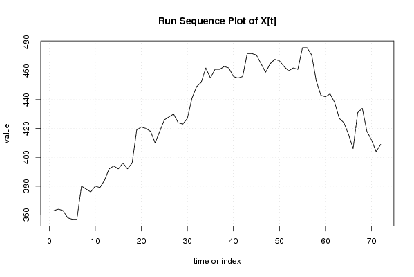
| Dataseries X: | |||||||||||||||||||||||||||||||||||||||||||||||||||||||||||||||||
363 364 363 358 357 357 380 378 376 380 379 384 392 394 392 396 392 396 419 421 420 418 410 418 426 428 430 424 423 427 441 449 452 462 455 461 461 463 462 456 455 456 472 472 471 465 459 465 468 467 463 460 462 461 476 476 471 453 443 442 444 438 427 424 416 406 431 434 418 412 404 409 | |||||||||||||||||||||||||||||||||||||||||||||||||||||||||||||||||
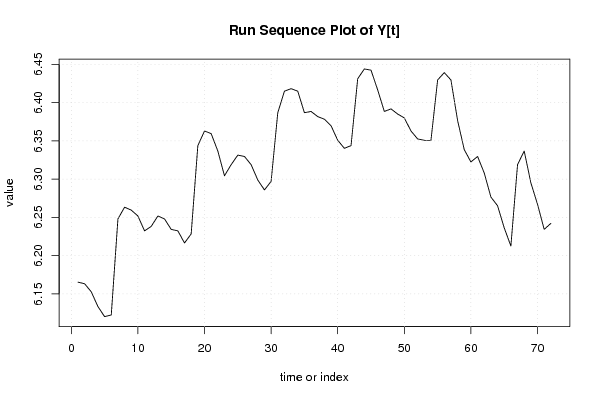
| Dataseries Y: | |||||||||||||||||||||||||||||||||||||||||||||||||||||||||||||||||
6,165417854 6,163314804 6,152732695 6,133398043 6,120297419 6,12249281 6,248042875 6,263398263 6,259581464 6,251903883 6,232448017 6,238324625 6,251903883 6,248042875 6,234410726 6,232448017 6,216606101 6,228511004 6,343880434 6,363028104 6,359573869 6,336825731 6,304448802 6,318968114 6,33150185 6,329720906 6,318968114 6,298949247 6,285998095 6,29710932 6,386879319 6,415096959 6,418364936 6,415096959 6,386879319 6,388561406 6,381816017 6,378426184 6,369900983 6,350885717 6,340359304 6,343880434 6,431331082 6,444131257 6,442540166 6,416732283 6,388561406 6,391917113 6,385194399 6,380122537 6,363028104 6,352629396 6,350885717 6,350885717 6,429719478 6,439350371 6,429719478 6,376726948 6,338594078 6,32256524 6,329720906 6,308098442 6,276643489 6,265301213 6,23636959 6,212606096 6,318968114 6,336825731 6,295266001 6,267200549 6,234410726 6,242223265 | |||||||||||||||||||||||||||||||||||||||||||||||||||||||||||||||||
Tables (Output of Computation) | |||||||||||||||||||||||||||||||||||||||||||||||||||||||||||||||||
| |||||||||||||||||||||||||||||||||||||||||||||||||||||||||||||||||
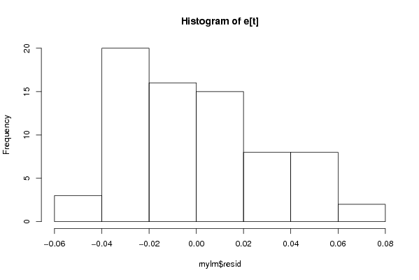
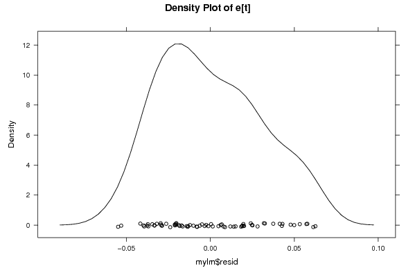
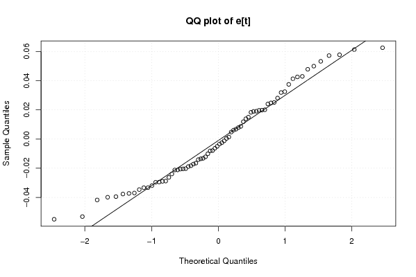
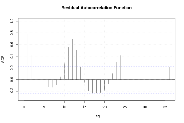
Figures (Output of Computation) | |||||||||||||||||||||||||||||||||||||||||||||||||||||||||||||||||
Input Parameters & R Code | |||||||||||||||||||||||||||||||||||||||||||||||||||||||||||||||||
| Parameters (Session): | |||||||||||||||||||||||||||||||||||||||||||||||||||||||||||||||||
| par1 = 50 ; par2 = 50 ; par3 = 0 ; par4 = 0 ; par5 = 0 ; par6 = Y ; par7 = Y ; | |||||||||||||||||||||||||||||||||||||||||||||||||||||||||||||||||
| Parameters (R input): | |||||||||||||||||||||||||||||||||||||||||||||||||||||||||||||||||
| par1 = 0 ; par2 = 36 ; | |||||||||||||||||||||||||||||||||||||||||||||||||||||||||||||||||
| R code (references can be found in the software module): | |||||||||||||||||||||||||||||||||||||||||||||||||||||||||||||||||
par1 <- as.numeric(par1) | |||||||||||||||||||||||||||||||||||||||||||||||||||||||||||||||||