Free Statistics
of Irreproducible Research!
Description of Statistical Computation | |||||||||||||||||||||||||||||||||||||||||||||||||||||||||||||||||
|---|---|---|---|---|---|---|---|---|---|---|---|---|---|---|---|---|---|---|---|---|---|---|---|---|---|---|---|---|---|---|---|---|---|---|---|---|---|---|---|---|---|---|---|---|---|---|---|---|---|---|---|---|---|---|---|---|---|---|---|---|---|---|---|---|---|
| Author's title | |||||||||||||||||||||||||||||||||||||||||||||||||||||||||||||||||
| Author | *The author of this computation has been verified* | ||||||||||||||||||||||||||||||||||||||||||||||||||||||||||||||||
| R Software Module | rwasp_edabi.wasp | ||||||||||||||||||||||||||||||||||||||||||||||||||||||||||||||||
| Title produced by software | Bivariate Explorative Data Analysis | ||||||||||||||||||||||||||||||||||||||||||||||||||||||||||||||||
| Date of computation | Fri, 30 Oct 2009 05:37:24 -0600 | ||||||||||||||||||||||||||||||||||||||||||||||||||||||||||||||||
| Cite this page as follows | Statistical Computations at FreeStatistics.org, Office for Research Development and Education, URL https://freestatistics.org/blog/index.php?v=date/2009/Oct/30/t1256903727le68ywdlkrx48b1.htm/, Retrieved Mon, 29 Apr 2024 05:01:37 +0000 | ||||||||||||||||||||||||||||||||||||||||||||||||||||||||||||||||
| Statistical Computations at FreeStatistics.org, Office for Research Development and Education, URL https://freestatistics.org/blog/index.php?pk=52080, Retrieved Mon, 29 Apr 2024 05:01:37 +0000 | |||||||||||||||||||||||||||||||||||||||||||||||||||||||||||||||||
| QR Codes: | |||||||||||||||||||||||||||||||||||||||||||||||||||||||||||||||||
|
| |||||||||||||||||||||||||||||||||||||||||||||||||||||||||||||||||
| Original text written by user: | |||||||||||||||||||||||||||||||||||||||||||||||||||||||||||||||||
| IsPrivate? | No (this computation is public) | ||||||||||||||||||||||||||||||||||||||||||||||||||||||||||||||||
| User-defined keywords | |||||||||||||||||||||||||||||||||||||||||||||||||||||||||||||||||
| Estimated Impact | 107 | ||||||||||||||||||||||||||||||||||||||||||||||||||||||||||||||||
Tree of Dependent Computations | |||||||||||||||||||||||||||||||||||||||||||||||||||||||||||||||||
| Family? (F = Feedback message, R = changed R code, M = changed R Module, P = changed Parameters, D = changed Data) | |||||||||||||||||||||||||||||||||||||||||||||||||||||||||||||||||
| - [Bivariate Explorative Data Analysis] [workshop 4,2,1] [2009-10-30 11:37:24] [2210215221105fab636491031ce54076] [Current] - D [Bivariate Explorative Data Analysis] [workshop 4,2,3] [2009-10-30 13:22:16] [35f0fff14d789f48983afb62e692bd0d] - RMPD [Trivariate Scatterplots] [workshop 5,1] [2009-10-30 14:16:01] [35f0fff14d789f48983afb62e692bd0d] - RMPD [Partial Correlation] [workshop 5,2] [2009-10-30 14:17:43] [35f0fff14d789f48983afb62e692bd0d] - RMPD [Bivariate Explorative Data Analysis] [workshop 5,3] [2009-11-04 20:21:14] [35f0fff14d789f48983afb62e692bd0d] - RMPD [Bivariate Explorative Data Analysis] [workshop 5,4] [2009-11-04 20:30:38] [35f0fff14d789f48983afb62e692bd0d] - RMPD [Bivariate Explorative Data Analysis] [workshop 5,5] [2009-11-04 20:39:02] [35f0fff14d789f48983afb62e692bd0d] | |||||||||||||||||||||||||||||||||||||||||||||||||||||||||||||||||
| Feedback Forum | |||||||||||||||||||||||||||||||||||||||||||||||||||||||||||||||||
Post a new message | |||||||||||||||||||||||||||||||||||||||||||||||||||||||||||||||||
Dataset | |||||||||||||||||||||||||||||||||||||||||||||||||||||||||||||||||
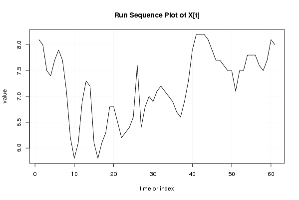
| Dataseries X: | |||||||||||||||||||||||||||||||||||||||||||||||||||||||||||||||||
8,1 8 7,5 7,4 7,7 7,9 7,7 7,1 6,2 5,8 6,1 6,9 7,3 7,2 6,1 5,8 6,1 6,3 6,8 6,8 6,5 6,2 6,3 6,4 6,6 7,6 6,4 6,8 7 6,9 7,1 7,2 7,1 7 6,9 6,7 6,6 6,9 7,3 7,9 8,2 8,2 8,2 8,1 7,9 7,7 7,7 7,6 7,5 7,5 7,1 7,5 7,5 7,8 7,8 7,8 7,6 7,5 7,7 8,1 8 | |||||||||||||||||||||||||||||||||||||||||||||||||||||||||||||||||
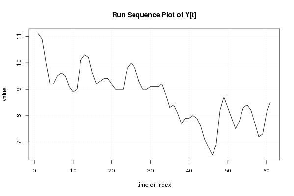
| Dataseries Y: | |||||||||||||||||||||||||||||||||||||||||||||||||||||||||||||||||
11,1 10,9 10 9,2 9,2 9,5 9,6 9,5 9,1 8,9 9 10,1 10,3 10,2 9,6 9,2 9,3 9,4 9,4 9,2 9 9 9 9,8 10 9,8 9,3 9 9 9,1 9,1 9,1 9,2 8,8 8,3 8,4 8,1 7,7 7,9 7,9 8 7,9 7,6 7,1 6,8 6,5 6,9 8,2 8,7 8,3 7,9 7,5 7,8 8,3 8,4 8,2 7,7 7,2 7,3 8,1 8,5 | |||||||||||||||||||||||||||||||||||||||||||||||||||||||||||||||||
Tables (Output of Computation) | |||||||||||||||||||||||||||||||||||||||||||||||||||||||||||||||||
| |||||||||||||||||||||||||||||||||||||||||||||||||||||||||||||||||
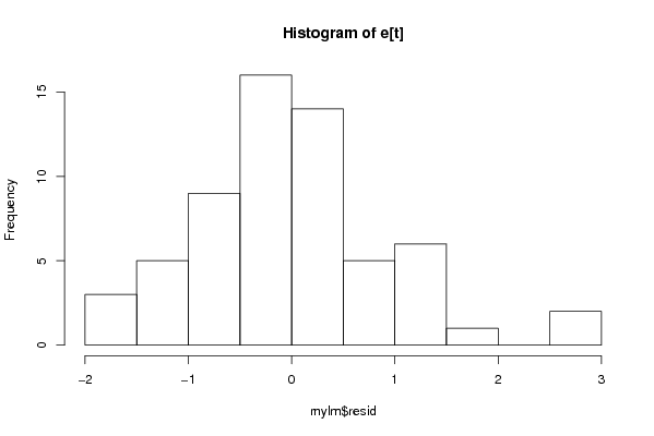
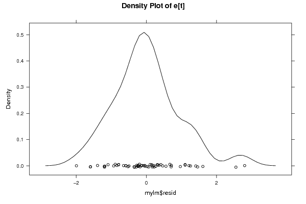
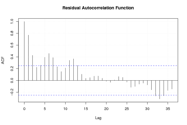
Figures (Output of Computation) | |||||||||||||||||||||||||||||||||||||||||||||||||||||||||||||||||
Input Parameters & R Code | |||||||||||||||||||||||||||||||||||||||||||||||||||||||||||||||||
| Parameters (Session): | |||||||||||||||||||||||||||||||||||||||||||||||||||||||||||||||||
| par1 = 0 ; par2 = 36 ; | |||||||||||||||||||||||||||||||||||||||||||||||||||||||||||||||||
| Parameters (R input): | |||||||||||||||||||||||||||||||||||||||||||||||||||||||||||||||||
| par1 = 0 ; par2 = 36 ; | |||||||||||||||||||||||||||||||||||||||||||||||||||||||||||||||||
| R code (references can be found in the software module): | |||||||||||||||||||||||||||||||||||||||||||||||||||||||||||||||||
par1 <- as.numeric(par1) | |||||||||||||||||||||||||||||||||||||||||||||||||||||||||||||||||