Free Statistics
of Irreproducible Research!
Description of Statistical Computation | |||||||||||||||||||||
|---|---|---|---|---|---|---|---|---|---|---|---|---|---|---|---|---|---|---|---|---|---|
| Author's title | |||||||||||||||||||||
| Author | *The author of this computation has been verified* | ||||||||||||||||||||
| R Software Module | rwasp_cloud.wasp | ||||||||||||||||||||
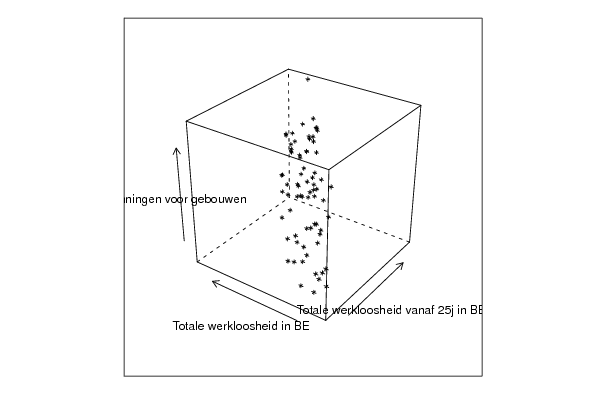
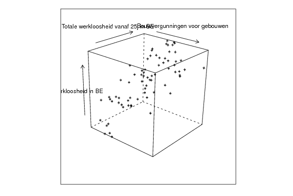
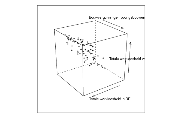
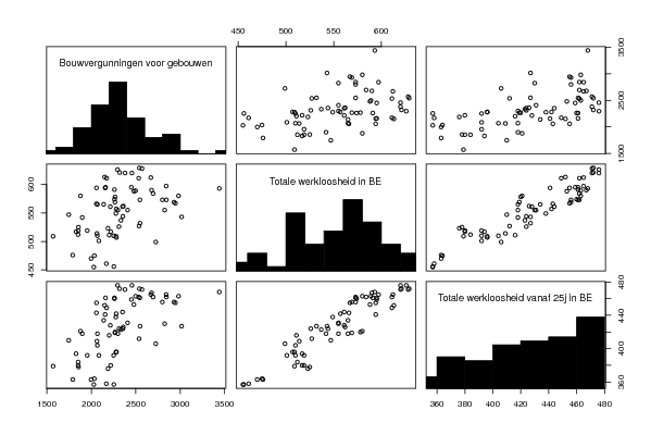
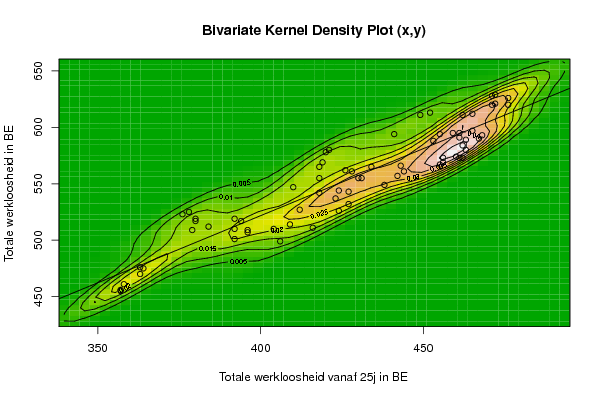
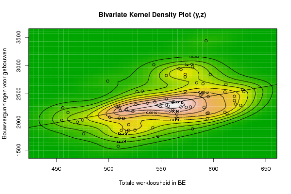
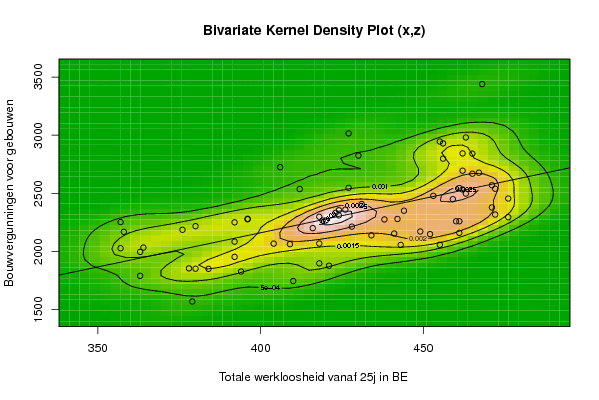
| Title produced by software | Trivariate Scatterplots | ||||||||||||||||||||
| Date of computation | Fri, 30 Oct 2009 07:22:48 -0600 | ||||||||||||||||||||
| Cite this page as follows | Statistical Computations at FreeStatistics.org, Office for Research Development and Education, URL https://freestatistics.org/blog/index.php?v=date/2009/Oct/30/t1256909135v1zo540dm8h20jk.htm/, Retrieved Mon, 29 Apr 2024 00:51:38 +0000 | ||||||||||||||||||||
| Statistical Computations at FreeStatistics.org, Office for Research Development and Education, URL https://freestatistics.org/blog/index.php?pk=52096, Retrieved Mon, 29 Apr 2024 00:51:38 +0000 | |||||||||||||||||||||
| QR Codes: | |||||||||||||||||||||
|
| |||||||||||||||||||||
| Original text written by user: | |||||||||||||||||||||
| IsPrivate? | No (this computation is public) | ||||||||||||||||||||
| User-defined keywords | |||||||||||||||||||||
| Estimated Impact | 164 | ||||||||||||||||||||
Tree of Dependent Computations | |||||||||||||||||||||
| Family? (F = Feedback message, R = changed R code, M = changed R Module, P = changed Parameters, D = changed Data) | |||||||||||||||||||||
| F [Univariate Data Series] [Gemiddelde renden...] [2008-10-13 19:42:56] [86c69698417c3ad89592e76776a2c65b] - PD [Univariate Data Series] [Bouwvergunningen ...] [2009-10-11 20:54:46] [5c968c05ca472afa314d272082b56b09] - RMPD [Trivariate Scatterplots] [WS5, Trivariate s...] [2009-10-30 13:22:48] [b8ce264f75295a954feffaf60221d1b0] [Current] | |||||||||||||||||||||
| Feedback Forum | |||||||||||||||||||||
Post a new message | |||||||||||||||||||||
Dataset | |||||||||||||||||||||
| Dataseries X: | |||||||||||||||||||||
363 364 363 358 357 357 380 378 376 380 379 384 392 394 392 396 392 396 419 421 420 418 410 418 426 428 430 424 423 427 441 449 452 462 455 461 461 463 462 456 455 456 472 472 471 465 459 465 468 467 463 460 462 461 476 476 471 453 443 442 444 438 427 424 416 406 431 434 418 412 404 409 | |||||||||||||||||||||
| Dataseries Y: | |||||||||||||||||||||
476 475 470 461 455 456 517 525 523 519 509 512 519 517 510 509 501 507 569 580 578 565 547 555 562 561 555 544 537 543 594 611 613 611 594 595 591 589 584 573 567 569 621 629 628 612 595 597 593 590 580 574 573 573 620 626 620 588 566 557 561 549 532 526 511 499 555 565 542 527 510 514 | |||||||||||||||||||||
| Dataseries Z: | |||||||||||||||||||||
1791 2034 1997 2169 2028 2253 2218 1855 2187 1852 1570 1851 1954 1828 2251 2277 2085 2282 2266 1878 2267 2069 1746 2299 2360 2214 2825 2355 2333 3016 2155 2172 2150 2533 2058 2160 2260 2498 2695 2799 2946 2930 2318 2540 2570 2669 2450 2842 3440 2678 2981 2260 2844 2546 2456 2295 2379 2479 2057 2280 2351 2276 2548 2311 2201 2725 2408 2139 1898 2537 2068 2063 | |||||||||||||||||||||
Tables (Output of Computation) | |||||||||||||||||||||
| |||||||||||||||||||||
Figures (Output of Computation) | |||||||||||||||||||||
Input Parameters & R Code | |||||||||||||||||||||
| Parameters (Session): | |||||||||||||||||||||
| par1 = 50 ; par2 = 50 ; par3 = Y ; par4 = Y ; par5 = Totale werkloosheid vanaf 25j in BE ; par6 = Totale werkloosheid in BE ; par7 = Bouwvergunningen voor gebouwen ; | |||||||||||||||||||||
| Parameters (R input): | |||||||||||||||||||||
| par1 = 50 ; par2 = 50 ; par3 = Y ; par4 = Y ; par5 = Totale werkloosheid vanaf 25j in BE ; par6 = Totale werkloosheid in BE ; par7 = Bouwvergunningen voor gebouwen ; | |||||||||||||||||||||
| R code (references can be found in the software module): | |||||||||||||||||||||
x <- array(x,dim=c(length(x),1)) | |||||||||||||||||||||