Free Statistics
of Irreproducible Research!
Description of Statistical Computation | |||||||||||||||||||||
|---|---|---|---|---|---|---|---|---|---|---|---|---|---|---|---|---|---|---|---|---|---|
| Author's title | |||||||||||||||||||||
| Author | *The author of this computation has been verified* | ||||||||||||||||||||
| R Software Module | rwasp_cloud.wasp | ||||||||||||||||||||
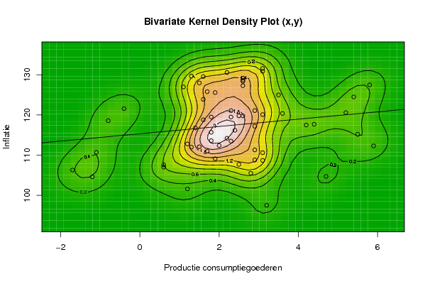
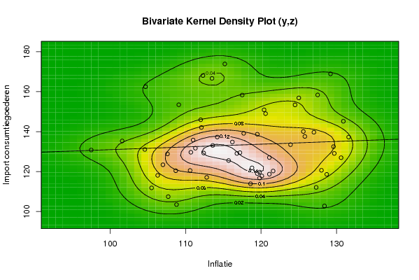
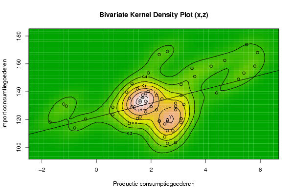
| Title produced by software | Trivariate Scatterplots | ||||||||||||||||||||
| Date of computation | Fri, 30 Oct 2009 08:19:10 -0600 | ||||||||||||||||||||
| Cite this page as follows | Statistical Computations at FreeStatistics.org, Office for Research Development and Education, URL https://freestatistics.org/blog/index.php?v=date/2009/Oct/30/t1256912405vhgnjha5oa57jns.htm/, Retrieved Mon, 29 Apr 2024 00:25:34 +0000 | ||||||||||||||||||||
| Statistical Computations at FreeStatistics.org, Office for Research Development and Education, URL https://freestatistics.org/blog/index.php?pk=52112, Retrieved Mon, 29 Apr 2024 00:25:34 +0000 | |||||||||||||||||||||
| QR Codes: | |||||||||||||||||||||
|
| |||||||||||||||||||||
| Original text written by user: | |||||||||||||||||||||
| IsPrivate? | No (this computation is public) | ||||||||||||||||||||
| User-defined keywords | |||||||||||||||||||||
| Estimated Impact | 202 | ||||||||||||||||||||
Tree of Dependent Computations | |||||||||||||||||||||
| Family? (F = Feedback message, R = changed R code, M = changed R Module, P = changed Parameters, D = changed Data) | |||||||||||||||||||||
| - [Univariate Data Series] [] [2009-10-13 19:25:20] [ff6896cd60d3b2257a9a5027c462fa18] - PD [Univariate Data Series] [SHWW2-Series2] [2009-10-13 19:36:05] [ff6896cd60d3b2257a9a5027c462fa18] - D [Univariate Data Series] [sHWW2-Series3] [2009-10-13 19:44:51] [ff6896cd60d3b2257a9a5027c462fa18] - RMPD [Trivariate Scatterplots] [SHWW5-1] [2009-10-30 14:19:10] [be285953263a374c1f072a85fb5ca13a] [Current] - RM D [Partial Correlation] [SHWW5-2] [2009-10-30 14:26:59] [ff6896cd60d3b2257a9a5027c462fa18] | |||||||||||||||||||||
| Feedback Forum | |||||||||||||||||||||
Post a new message | |||||||||||||||||||||
Dataset | |||||||||||||||||||||
| Dataseries X: | |||||||||||||||||||||
2.9 2.6 2.3 2.3 2.6 3.1 2.8 2.5 2.9 3.1 3.1 3.2 2.5 2.6 2.9 2.6 2.4 1.7 2 2.2 1.9 1.6 1.6 1.2 1.2 1.5 1.6 1.7 1.8 1.8 1.8 1.3 1.3 1.4 1.1 1.5 2.2 2.9 3.1 3.5 3.6 4.4 4.2 5.2 5.8 5.9 5.4 5.5 4.7 3.1 2.6 2.3 1.9 0.6 0.6 -0.4 -1.1 -1.7 -0.8 -1.2 | |||||||||||||||||||||
| Dataseries Y: | |||||||||||||||||||||
108.8 128.4 121.1 119.5 128.7 108.7 105.5 119.8 111.3 110.6 120.1 97.5 107.7 127.3 117.2 119.8 116.2 111 112.4 130.6 109.1 118.8 123.9 101.6 112.8 128 129.6 125.8 119.5 115.7 113.6 129.7 112 116.8 127 112.1 114.2 121.1 131.6 125 120.4 117.7 117.5 120.6 127.5 112.3 124.5 115.2 104.7 130.9 129.2 113.5 125.6 107.6 107 121.6 110.7 106.3 118.6 104.6 | |||||||||||||||||||||
| Dataseries Z: | |||||||||||||||||||||
103.5 102.8 118.72 119.01 118.61 120.43 111.83 116.79 131.71 120.57 117.83 130.8 107.46 112.09 129.47 119.72 134.81 135.8 129.27 126.94 153.45 121.86 133.47 135.34 117.1 120.65 132.49 137.6 138.69 125.53 133.09 129.08 145.94 129.07 139.69 142.09 137.29 127.03 137.25 156.87 150.89 139.14 158.3 149 158.36 168.06 153.38 173.86 162.47 145.17 168.89 166.64 140.07 128.84 123.41 120.3 129.67 118.1 113.91 131.09 | |||||||||||||||||||||
Tables (Output of Computation) | |||||||||||||||||||||
| |||||||||||||||||||||
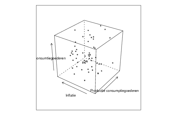
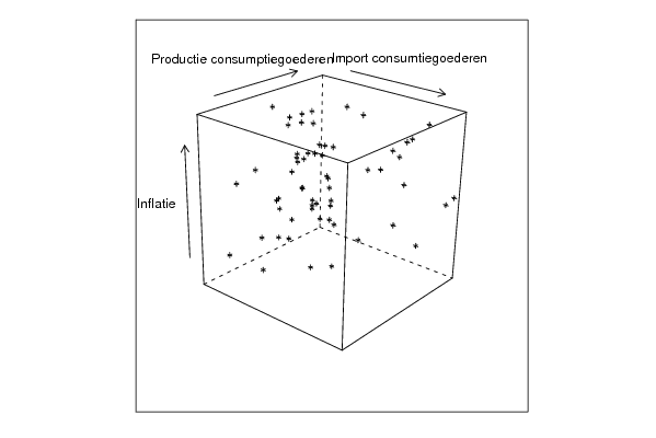
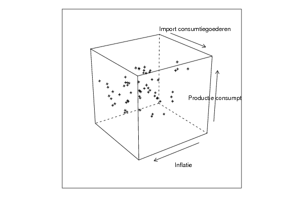
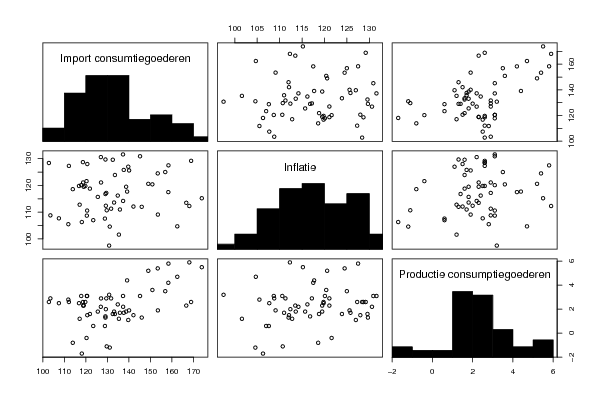
Figures (Output of Computation) | |||||||||||||||||||||
Input Parameters & R Code | |||||||||||||||||||||
| Parameters (Session): | |||||||||||||||||||||
| par1 = 0 ; par2 = 36 ; | |||||||||||||||||||||
| Parameters (R input): | |||||||||||||||||||||
| par1 = 50 ; par2 = 50 ; par3 = Y ; par4 = Y ; par5 = Productie consumptiegoederen ; par6 = Inflatie ; par7 = Import consumtiegoederen ; | |||||||||||||||||||||
| R code (references can be found in the software module): | |||||||||||||||||||||
x <- array(x,dim=c(length(x),1)) | |||||||||||||||||||||