Free Statistics
of Irreproducible Research!
Description of Statistical Computation | |||||||||||||||||||||
|---|---|---|---|---|---|---|---|---|---|---|---|---|---|---|---|---|---|---|---|---|---|
| Author's title | |||||||||||||||||||||
| Author | *Unverified author* | ||||||||||||||||||||
| R Software Module | rwasp_meanplot.wasp | ||||||||||||||||||||
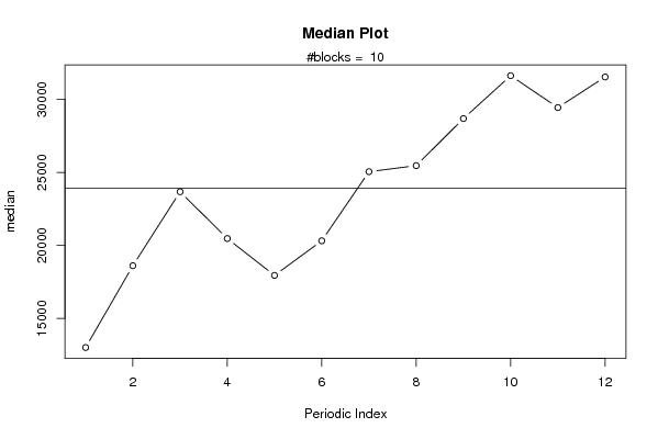
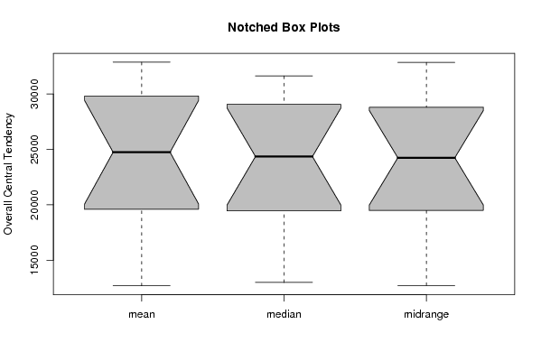
| Title produced by software | Mean Plot | ||||||||||||||||||||
| Date of computation | Mon, 26 Apr 2010 21:57:04 +0000 | ||||||||||||||||||||
| Cite this page as follows | Statistical Computations at FreeStatistics.org, Office for Research Development and Education, URL https://freestatistics.org/blog/index.php?v=date/2010/Apr/26/t12723190683ranzaz9g8h985l.htm/, Retrieved Sat, 27 Jul 2024 06:28:20 +0000 | ||||||||||||||||||||
| Statistical Computations at FreeStatistics.org, Office for Research Development and Education, URL https://freestatistics.org/blog/index.php?pk=74922, Retrieved Sat, 27 Jul 2024 06:28:20 +0000 | |||||||||||||||||||||
| QR Codes: | |||||||||||||||||||||
|
| |||||||||||||||||||||
| Original text written by user: | |||||||||||||||||||||
| IsPrivate? | No (this computation is public) | ||||||||||||||||||||
| User-defined keywords | KDGP2W12 | ||||||||||||||||||||
| Estimated Impact | 200 | ||||||||||||||||||||
Tree of Dependent Computations | |||||||||||||||||||||
| Family? (F = Feedback message, R = changed R code, M = changed R Module, P = changed Parameters, D = changed Data) | |||||||||||||||||||||
| - [Histogram] [Datareeks-Inschri...] [2010-02-08 14:03:15] [c656187b38b4f6e6948d94f8dfe6ded2] - RMP [Harrell-Davis Quantiles] [Datareeks-Opdrach...] [2010-03-08 17:35:01] [1f3241a8f2363a866734862cbbf73252] - RMPD [Mean Plot] [Opgave 6 oefening...] [2010-04-26 21:57:04] [8c87877ca0a068b5d9f0f8fa9cf6c0e7] [Current] - D [Mean Plot] [Opgave 6 oefening...] [2010-04-28 15:35:23] [1f3241a8f2363a866734862cbbf73252] - RMPD [(Partial) Autocorrelation Function] [Opgave 6 BIS oefe...] [2010-05-03 18:06:05] [1f3241a8f2363a866734862cbbf73252] - P [(Partial) Autocorrelation Function] [Opgave 6 BIS oefe...] [2010-05-03 18:08:48] [1f3241a8f2363a866734862cbbf73252] - P [(Partial) Autocorrelation Function] [Opgave 6 BIS oefe...] [2010-05-03 18:11:43] [1f3241a8f2363a866734862cbbf73252] - P [(Partial) Autocorrelation Function] [Opgave 6 BIS oefe...] [2010-05-03 18:13:08] [1f3241a8f2363a866734862cbbf73252] | |||||||||||||||||||||
| Feedback Forum | |||||||||||||||||||||
Post a new message | |||||||||||||||||||||
Dataset | |||||||||||||||||||||
| Dataseries X: | |||||||||||||||||||||
14538 18730 22485 20036 16971 19028 22759 20516 26195 27786 24090 25447 11509 15572 22518 20520 17789 20205 26835 25826 31934 30019 30111 31566 12738 19814 24776 20424 18688 20418 25778 25100 25859 30651 26551 31124 9367 17382 20995 18205 17328 18157 23691 26736 27165 34506 29506 31956 10698 18479 19785 19684 18730 17970 27044 22405 26482 29096 25591 29743 13807 19169 22782 20366 17537 18004 24319 22679 32034 36438 29383 28029 15548 17704 25316 20764 18089 21705 23843 22397 26105 29462 27071 31514 11514 17409 24561 21382 17351 22780 23970 26887 34777 35022 35338 36845 13971 22228 28806 20506 22414 25814 28352 29965 30212 32609 30364 37702 13253 21790 27192 21725 22205 24693 29133 35953 37863 43129 39690 41086 | |||||||||||||||||||||
Tables (Output of Computation) | |||||||||||||||||||||
| |||||||||||||||||||||
Figures (Output of Computation) | |||||||||||||||||||||
Input Parameters & R Code | |||||||||||||||||||||
| Parameters (Session): | |||||||||||||||||||||
| par1 = 12 ; | |||||||||||||||||||||
| Parameters (R input): | |||||||||||||||||||||
| par1 = 12 ; | |||||||||||||||||||||
| R code (references can be found in the software module): | |||||||||||||||||||||
par1 <- as.numeric(par1) | |||||||||||||||||||||