Free Statistics
of Irreproducible Research!
Description of Statistical Computation | |||||||||||||||||||||||||||||||||||||||||||||||||||||||||||||||||||||||||||||||||||||||||||||||||||||||||||||||||||||||||||||||||||||||||||||||||||||||||||||||||||||||||
|---|---|---|---|---|---|---|---|---|---|---|---|---|---|---|---|---|---|---|---|---|---|---|---|---|---|---|---|---|---|---|---|---|---|---|---|---|---|---|---|---|---|---|---|---|---|---|---|---|---|---|---|---|---|---|---|---|---|---|---|---|---|---|---|---|---|---|---|---|---|---|---|---|---|---|---|---|---|---|---|---|---|---|---|---|---|---|---|---|---|---|---|---|---|---|---|---|---|---|---|---|---|---|---|---|---|---|---|---|---|---|---|---|---|---|---|---|---|---|---|---|---|---|---|---|---|---|---|---|---|---|---|---|---|---|---|---|---|---|---|---|---|---|---|---|---|---|---|---|---|---|---|---|---|---|---|---|---|---|---|---|---|---|---|---|---|---|---|---|---|
| Author's title | |||||||||||||||||||||||||||||||||||||||||||||||||||||||||||||||||||||||||||||||||||||||||||||||||||||||||||||||||||||||||||||||||||||||||||||||||||||||||||||||||||||||||
| Author | *The author of this computation has been verified* | ||||||||||||||||||||||||||||||||||||||||||||||||||||||||||||||||||||||||||||||||||||||||||||||||||||||||||||||||||||||||||||||||||||||||||||||||||||||||||||||||||||||||
| R Software Module | Ian.Hollidayrwasp_Simple Regression Y ~ X.wasp | ||||||||||||||||||||||||||||||||||||||||||||||||||||||||||||||||||||||||||||||||||||||||||||||||||||||||||||||||||||||||||||||||||||||||||||||||||||||||||||||||||||||||
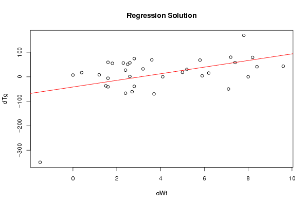
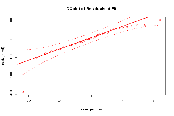
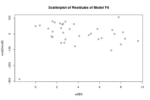
| Title produced by software | Simple Linear Regression | ||||||||||||||||||||||||||||||||||||||||||||||||||||||||||||||||||||||||||||||||||||||||||||||||||||||||||||||||||||||||||||||||||||||||||||||||||||||||||||||||||||||||
| Date of computation | Wed, 28 Apr 2010 07:33:16 +0000 | ||||||||||||||||||||||||||||||||||||||||||||||||||||||||||||||||||||||||||||||||||||||||||||||||||||||||||||||||||||||||||||||||||||||||||||||||||||||||||||||||||||||||
| Cite this page as follows | Statistical Computations at FreeStatistics.org, Office for Research Development and Education, URL https://freestatistics.org/blog/index.php?v=date/2010/Apr/28/t1272440394xivdpwjvfmulga6.htm/, Retrieved Tue, 30 Apr 2024 19:01:25 +0000 | ||||||||||||||||||||||||||||||||||||||||||||||||||||||||||||||||||||||||||||||||||||||||||||||||||||||||||||||||||||||||||||||||||||||||||||||||||||||||||||||||||||||||
| Statistical Computations at FreeStatistics.org, Office for Research Development and Education, URL https://freestatistics.org/blog/index.php?pk=74949, Retrieved Tue, 30 Apr 2024 19:01:25 +0000 | |||||||||||||||||||||||||||||||||||||||||||||||||||||||||||||||||||||||||||||||||||||||||||||||||||||||||||||||||||||||||||||||||||||||||||||||||||||||||||||||||||||||||
| QR Codes: | |||||||||||||||||||||||||||||||||||||||||||||||||||||||||||||||||||||||||||||||||||||||||||||||||||||||||||||||||||||||||||||||||||||||||||||||||||||||||||||||||||||||||
|
| |||||||||||||||||||||||||||||||||||||||||||||||||||||||||||||||||||||||||||||||||||||||||||||||||||||||||||||||||||||||||||||||||||||||||||||||||||||||||||||||||||||||||
| Original text written by user: | Data from the STARS database http://stars.ac.uk/index.php | ||||||||||||||||||||||||||||||||||||||||||||||||||||||||||||||||||||||||||||||||||||||||||||||||||||||||||||||||||||||||||||||||||||||||||||||||||||||||||||||||||||||||
| IsPrivate? | No (this computation is public) | ||||||||||||||||||||||||||||||||||||||||||||||||||||||||||||||||||||||||||||||||||||||||||||||||||||||||||||||||||||||||||||||||||||||||||||||||||||||||||||||||||||||||
| User-defined keywords | Triglyceride, weight loss, linear regression | ||||||||||||||||||||||||||||||||||||||||||||||||||||||||||||||||||||||||||||||||||||||||||||||||||||||||||||||||||||||||||||||||||||||||||||||||||||||||||||||||||||||||
| Estimated Impact | 296 | ||||||||||||||||||||||||||||||||||||||||||||||||||||||||||||||||||||||||||||||||||||||||||||||||||||||||||||||||||||||||||||||||||||||||||||||||||||||||||||||||||||||||
Tree of Dependent Computations | |||||||||||||||||||||||||||||||||||||||||||||||||||||||||||||||||||||||||||||||||||||||||||||||||||||||||||||||||||||||||||||||||||||||||||||||||||||||||||||||||||||||||
| Family? (F = Feedback message, R = changed R code, M = changed R Module, P = changed Parameters, D = changed Data) | |||||||||||||||||||||||||||||||||||||||||||||||||||||||||||||||||||||||||||||||||||||||||||||||||||||||||||||||||||||||||||||||||||||||||||||||||||||||||||||||||||||||||
| - [Simple Linear Regression] [PY2224 Mock Exam ...] [2010-04-28 07:33:16] [a9208f4f8d3b118336aae915785f2bd9] [Current] - RMPD [Correlation] [PY2224 Mock Exam ...] [2010-04-28 07:52:28] [98fd0e87c3eb04e0cc2efde01dbafab6] - [Correlation] [PY2224 Mock Exam ...] [2010-04-28 08:03:45] [98fd0e87c3eb04e0cc2efde01dbafab6] - M D [Correlation] [PY2224 May Mock E...] [2010-04-28 12:25:43] [98fd0e87c3eb04e0cc2efde01dbafab6] - D [Correlation] [PY2224 May Mock E...] [2010-04-30 11:35:53] [98fd0e87c3eb04e0cc2efde01dbafab6] - D [Correlation] [] [2010-05-04 13:10:21] [82439cd473f0ddf8a88eb1802dda9b6c] - D [Correlation] [] [2010-05-04 13:07:45] [e8bb49267f0b4e611f4778412d0811f2] - D [Correlation] [Mockexam1] [2010-05-04 13:09:19] [226e457c23f16abdaf22fe48e6e411fd] - D [Correlation] [Correlation of tr...] [2010-05-04 13:12:24] [f0a7b9ce333a507984a56d87311bd9a6] - D [Correlation] [Mock] [2010-05-04 13:15:09] [d85e8cd4dd2ccdf2c3dfa3761837f774] - D [Correlation] [Correlation of Tr...] [2010-05-04 13:14:23] [7756e15f439c0db38d660c862abbb747] - D [Correlation] [Correlation graph...] [2010-05-04 13:15:47] [991f3c16ff1ec6689e9f3866d072593e] - D [Correlation] [correlation] [2010-05-04 13:15:13] [c7d0e78e2fa8da0e0b2bee0011c20ac0] - D [Correlation] [mockexam] [2010-05-04 13:16:50] [66f61a2d5ef80b1eafe31e5651ad0889] - D [Correlation] [triglyceride vs w...] [2010-05-04 13:15:36] [a58114c03403c4a3c11c78968b4ee919] - D [Correlation] [triglyceride leve...] [2010-05-04 13:17:15] [2185b0545466c0a8649e1b1b76e104e0] - D [Correlation] [question 2 1] [2010-05-04 13:14:55] [256a42577f5eb7e9c8a1b74c73a90fa8] - D [Correlation] [] [2010-05-04 13:15:11] [5cae40017fc37cfe76436682b5003098] - [Correlation] [mock correlation] [2010-05-04 13:18:20] [153000c0b3bd367036e4d581452d08df] - [Correlation] [mock correlation] [2010-05-04 13:18:20] [153000c0b3bd367036e4d581452d08df] - D [Correlation] [] [2010-05-04 13:18:55] [609c1e5ad6fe9b179b6d83d13356f854] - D [Correlation] [Stats mock] [2010-05-04 13:20:06] [012a64ac316c94a67eaef3285dac2cf7] - D [Correlation] [mock exam comp1] [2010-05-04 13:17:06] [0dff2a868db4b5bcbf64703b84410784] - D [Correlation] [mock exam 1] [2010-05-04 13:20:20] [74be16979710d4c4e7c6647856088456] - D [Correlation] [] [2010-05-04 13:14:09] [bc03f19b1cbb14de25d671293ac6c773] - D [Correlation] [Mock ii] [2010-05-04 13:21:20] [856c65906cd78e3f7881668c6dfea87f] - D [Correlation] [ii] [2010-05-04 13:13:13] [885328d98a95a442af53d0763bccf325] - D [Correlation] [Basline correlation] [2010-05-04 13:21:45] [74be16979710d4c4e7c6647856088456] - D [Correlation] [Graph 1] [2010-05-04 13:23:28] [c519646407a489a26f129bdc22b2e203] - P [Correlation] [graph 2] [2010-05-04 14:33:27] [c519646407a489a26f129bdc22b2e203] - D [Correlation] [] [2010-05-04 13:23:40] [74be16979710d4c4e7c6647856088456] - D [Correlation] [Correlation betwe...] [2010-05-04 13:23:56] [991f3c16ff1ec6689e9f3866d072593e] - PD [Correlation] [obeisty study] [2010-05-04 13:23:18] [74be16979710d4c4e7c6647856088456] - [Correlation] [A graph to show c...] [2010-05-04 13:10:46] [a04c3705631ba28c4a7ea7999bc2469c] - PD [Correlation] [Weight] [2010-05-04 13:23:12] [31938d087c55cf67127a01ef1e8f38ba] - D [Correlation] [] [2010-05-04 13:20:43] [7ee8584ae92dbbc2a823887b8397aaa8] - D [Correlation] [question 2 2 ] [2010-05-04 13:26:22] [256a42577f5eb7e9c8a1b74c73a90fa8] - D [Correlation] [mock] [2010-05-04 13:15:22] [9071c1a88a977c8c2dd0accff6b1d644] - D [Correlation] [] [2010-05-04 13:25:33] [226e457c23f16abdaf22fe48e6e411fd] - [Correlation] [] [2010-05-04 13:17:25] [0848a45f8a904661abc16c2a3570ded4] - D [Correlation] [correlation of ch...] [2010-05-04 13:21:40] [a2ec18f77143ca7c2255feafca790c81] - D [Correlation] [] [2010-05-04 13:19:53] [869dc8c90da15910a169a569d8b6a5c9] - D [Correlation] [correlation of ch...] [2010-05-04 13:21:40] [a2ec18f77143ca7c2255feafca790c81] - D [Correlation] [Correlation week 8 ] [2010-05-04 13:27:21] [74be16979710d4c4e7c6647856088456] - D [Correlation] [Mock exam ] [2010-05-04 13:27:05] [efb93495a892eea584966de4a02d2ce4] - D [Correlation] [Correlation ] [2010-05-04 13:25:09] [da3db4ee336105e3f28c420d1eeb41bc] - D [Correlation] [correlation] [2010-05-04 13:21:11] [9dc333cea70095e4d9c08ad15f70f6c6] - D [Correlation] [] [2010-05-04 13:25:51] [a120050d9c71216a504f7d26958aa6f2] - D [Correlation] [exam - correlatio...] [2010-05-04 13:25:20] [6754037f2a7547483397efade45eb176] [Truncated] | |||||||||||||||||||||||||||||||||||||||||||||||||||||||||||||||||||||||||||||||||||||||||||||||||||||||||||||||||||||||||||||||||||||||||||||||||||||||||||||||||||||||||
| Feedback Forum | |||||||||||||||||||||||||||||||||||||||||||||||||||||||||||||||||||||||||||||||||||||||||||||||||||||||||||||||||||||||||||||||||||||||||||||||||||||||||||||||||||||||||
Post a new message | |||||||||||||||||||||||||||||||||||||||||||||||||||||||||||||||||||||||||||||||||||||||||||||||||||||||||||||||||||||||||||||||||||||||||||||||||||||||||||||||||||||||||
Dataset | |||||||||||||||||||||||||||||||||||||||||||||||||||||||||||||||||||||||||||||||||||||||||||||||||||||||||||||||||||||||||||||||||||||||||||||||||||||||||||||||||||||||||
| Dataseries X: | |||||||||||||||||||||||||||||||||||||||||||||||||||||||||||||||||||||||||||||||||||||||||||||||||||||||||||||||||||||||||||||||||||||||||||||||||||||||||||||||||||||||||
1.6 -41.0 1.8 55.0 5.2 30.0 4.1 0.0 0.4 17.0 2.7 -61.0 2.4 27.0 2.6 1.0 2.4 -67.0 7.2 80.0 3.7 -70.0 8.4 41.0 1.5 -37.0 8.0 0.0 0.0 7.0 7.1 -50.0 2.8 74.0 8.2 79.0 2.3 56.0 5.0 18.0 5.9 4.0 6.2 15.0 3.6 69.0 1.6 -6.0 3.2 32.0 2.6 57.0 1.6 59.0 5.8 68.0 2.8 -39.0 1.2 8.0 -1.5 -349.0 7.8 169.0 2.5 51.0 9.6 43.0 7.4 58.0 | |||||||||||||||||||||||||||||||||||||||||||||||||||||||||||||||||||||||||||||||||||||||||||||||||||||||||||||||||||||||||||||||||||||||||||||||||||||||||||||||||||||||||
Tables (Output of Computation) | |||||||||||||||||||||||||||||||||||||||||||||||||||||||||||||||||||||||||||||||||||||||||||||||||||||||||||||||||||||||||||||||||||||||||||||||||||||||||||||||||||||||||
| |||||||||||||||||||||||||||||||||||||||||||||||||||||||||||||||||||||||||||||||||||||||||||||||||||||||||||||||||||||||||||||||||||||||||||||||||||||||||||||||||||||||||
Figures (Output of Computation) | |||||||||||||||||||||||||||||||||||||||||||||||||||||||||||||||||||||||||||||||||||||||||||||||||||||||||||||||||||||||||||||||||||||||||||||||||||||||||||||||||||||||||
Input Parameters & R Code | |||||||||||||||||||||||||||||||||||||||||||||||||||||||||||||||||||||||||||||||||||||||||||||||||||||||||||||||||||||||||||||||||||||||||||||||||||||||||||||||||||||||||
| Parameters (Session): | |||||||||||||||||||||||||||||||||||||||||||||||||||||||||||||||||||||||||||||||||||||||||||||||||||||||||||||||||||||||||||||||||||||||||||||||||||||||||||||||||||||||||
| par1 = 2 ; par2 = 1 ; par3 = TRUE ; | |||||||||||||||||||||||||||||||||||||||||||||||||||||||||||||||||||||||||||||||||||||||||||||||||||||||||||||||||||||||||||||||||||||||||||||||||||||||||||||||||||||||||
| Parameters (R input): | |||||||||||||||||||||||||||||||||||||||||||||||||||||||||||||||||||||||||||||||||||||||||||||||||||||||||||||||||||||||||||||||||||||||||||||||||||||||||||||||||||||||||
| par1 = 2 ; par2 = 1 ; par3 = TRUE ; | |||||||||||||||||||||||||||||||||||||||||||||||||||||||||||||||||||||||||||||||||||||||||||||||||||||||||||||||||||||||||||||||||||||||||||||||||||||||||||||||||||||||||
| R code (references can be found in the software module): | |||||||||||||||||||||||||||||||||||||||||||||||||||||||||||||||||||||||||||||||||||||||||||||||||||||||||||||||||||||||||||||||||||||||||||||||||||||||||||||||||||||||||
cat1 <- as.numeric(par1) # | |||||||||||||||||||||||||||||||||||||||||||||||||||||||||||||||||||||||||||||||||||||||||||||||||||||||||||||||||||||||||||||||||||||||||||||||||||||||||||||||||||||||||