Free Statistics
of Irreproducible Research!
Description of Statistical Computation | |||||||||||||||||||||||||||||||||||||||||||||||||||||
|---|---|---|---|---|---|---|---|---|---|---|---|---|---|---|---|---|---|---|---|---|---|---|---|---|---|---|---|---|---|---|---|---|---|---|---|---|---|---|---|---|---|---|---|---|---|---|---|---|---|---|---|---|---|
| Author's title | |||||||||||||||||||||||||||||||||||||||||||||||||||||
| Author | *The author of this computation has been verified* | ||||||||||||||||||||||||||||||||||||||||||||||||||||
| R Software Module | rwasp_edauni.wasp | ||||||||||||||||||||||||||||||||||||||||||||||||||||
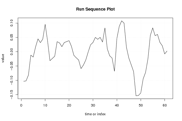
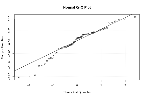
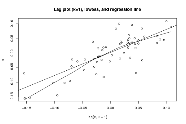
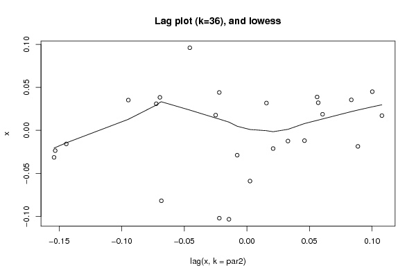
| Title produced by software | Univariate Explorative Data Analysis | ||||||||||||||||||||||||||||||||||||||||||||||||||||
| Date of computation | Tue, 21 Dec 2010 12:18:24 +0000 | ||||||||||||||||||||||||||||||||||||||||||||||||||||
| Cite this page as follows | Statistical Computations at FreeStatistics.org, Office for Research Development and Education, URL https://freestatistics.org/blog/index.php?v=date/2010/Dec/21/t1292933785ixww88i6vfw4may.htm/, Retrieved Fri, 17 May 2024 21:07:34 +0000 | ||||||||||||||||||||||||||||||||||||||||||||||||||||
| Statistical Computations at FreeStatistics.org, Office for Research Development and Education, URL https://freestatistics.org/blog/index.php?pk=113370, Retrieved Fri, 17 May 2024 21:07:34 +0000 | |||||||||||||||||||||||||||||||||||||||||||||||||||||
| QR Codes: | |||||||||||||||||||||||||||||||||||||||||||||||||||||
|
| |||||||||||||||||||||||||||||||||||||||||||||||||||||
| Original text written by user: | |||||||||||||||||||||||||||||||||||||||||||||||||||||
| IsPrivate? | No (this computation is public) | ||||||||||||||||||||||||||||||||||||||||||||||||||||
| User-defined keywords | |||||||||||||||||||||||||||||||||||||||||||||||||||||
| Estimated Impact | 132 | ||||||||||||||||||||||||||||||||||||||||||||||||||||
Tree of Dependent Computations | |||||||||||||||||||||||||||||||||||||||||||||||||||||
| Family? (F = Feedback message, R = changed R code, M = changed R Module, P = changed Parameters, D = changed Data) | |||||||||||||||||||||||||||||||||||||||||||||||||||||
| - [Univariate Explorative Data Analysis] [b-r0245787] [2010-12-19 16:05:46] [ebb35fb07def4d07c0eb7ec8d2fd3b0e] - D [Univariate Explorative Data Analysis] [b-r0245095] [2010-12-19 16:19:41] [ec8d68d52c1e9c5e97bb689b42436a8c] - D [Univariate Explorative Data Analysis] [b-r0245095] [2010-12-21 10:45:43] [ec8d68d52c1e9c5e97bb689b42436a8c] - D [Univariate Explorative Data Analysis] [b-r0245095] [2010-12-21 12:18:24] [4bfaadb29d89ff24ebcdd4f425066435] [Current] | |||||||||||||||||||||||||||||||||||||||||||||||||||||
| Feedback Forum | |||||||||||||||||||||||||||||||||||||||||||||||||||||
Post a new message | |||||||||||||||||||||||||||||||||||||||||||||||||||||
Dataset | |||||||||||||||||||||||||||||||||||||||||||||||||||||
| Dataseries X: | |||||||||||||||||||||||||||||||||||||||||||||||||||||
-0.103395775413547 -0.102119071477734 -0.0818766243906285 -0.0119800214843379 -0.0186348038511091 0.0171247716603502 0.0449528608692251 0.0317466932293922 0.0440576540139132 0.0960227706176194 0.0383337314021404 -0.0314238215107543 -0.0235957323018794 -0.0157676430930045 0.0351632166619939 0.0309227921734532 0.0177166245336203 0.0320960990155569 0.0354413166487858 0.0387865342820146 0.0186831371883051 -0.0124545167541122 -0.021177812818299 -0.0288668520337780 -0.0589702491274875 -0.0466592883429665 -0.0288311991340916 -0.00100310992521664 0.0244106214054278 0.0322387106143028 0.0500667998231777 0.0434120174564065 0.0502058498165736 0.0338969116306172 0.0831051018690146 0.00989893422918181 -0.0143414902593589 -0.0220305294748379 -0.0683394676607944 0.0460400068211422 0.088696811786478 0.107905002024876 0.100215962809397 0.0156296941400409 -0.0220593450754381 -0.0456113568960858 -0.0695092128975482 -0.154095481566904 -0.153164621811905 -0.144302275754323 -0.0947515170288468 -0.0724405562443258 -0.0249583112162656 0.0570068053874405 0.0834547935667928 0.0561115985321286 0.0604910730140652 0.0328020337985862 0.0209759671882759 -0.00774732887591092 0.00249511821119445 | |||||||||||||||||||||||||||||||||||||||||||||||||||||
Tables (Output of Computation) | |||||||||||||||||||||||||||||||||||||||||||||||||||||
| |||||||||||||||||||||||||||||||||||||||||||||||||||||
Figures (Output of Computation) | |||||||||||||||||||||||||||||||||||||||||||||||||||||
Input Parameters & R Code | |||||||||||||||||||||||||||||||||||||||||||||||||||||
| Parameters (Session): | |||||||||||||||||||||||||||||||||||||||||||||||||||||
| par1 = 0 ; par2 = 36 ; | |||||||||||||||||||||||||||||||||||||||||||||||||||||
| Parameters (R input): | |||||||||||||||||||||||||||||||||||||||||||||||||||||
| par1 = 0 ; par2 = 36 ; | |||||||||||||||||||||||||||||||||||||||||||||||||||||
| R code (references can be found in the software module): | |||||||||||||||||||||||||||||||||||||||||||||||||||||
par1 <- as.numeric(par1) | |||||||||||||||||||||||||||||||||||||||||||||||||||||