Free Statistics

of Irreproducible Research!

Author's title

Author*Unverified author*
R Software Modulerwasp_Reddy-Moores Data Boxplot.wasp
Title produced by softwareBoxplot and Trimmed Means
Date of computationWed, 02 Jun 2010 09:46:12 +0000
Cite this page as followsStatistical Computations at FreeStatistics.org, Office for Research Development and Education, URL https://freestatistics.org/blog/index.php?v=date/2010/Jun/02/t1275471999gaaoqhc59zv2zyl.htm/, Retrieved Sat, 20 Apr 2024 08:24:25 +0000
Statistical Computations at FreeStatistics.org, Office for Research Development and Education, URL https://freestatistics.org/blog/index.php?pk=77065, Retrieved Sat, 20 Apr 2024 08:24:25 +0000
QR Codes:

Original text written by user:
IsPrivate?No (this computation is public)
User-defined keywords
Estimated Impact132
Family? (F = Feedback message, R = changed R code, M = changed R Module, P = changed Parameters, D = changed Data)
-     [Histogram and QQplot] [PY2224 Aston Work...] [2009-10-06 09:57:09] [98fd0e87c3eb04e0cc2efde01dbafab6]
-   P   [Histogram and QQplot] [Histogram and QQPlot] [2009-10-12 19:58:08] [cefd16489930d37792a2dfe143e1dd64]
- RMPD      [Boxplot and Trimmed Means] [] [2010-06-02 09:46:12] [08805e86e61bf35728943c4aec6d6f47] [Current]
- RMPD        [T-Tests] [] [2010-06-02 09:55:47] [981ccd4f0082ace49a11aa7a2b792a9c]
Feedback Forum

Post a new message
Dataseries X:
-1.1
-3.5
1
-0.1
-0.4
-3.7
0.4
-5.9
-1.4
-0.9
-0.6
1
-1.6
-0.5
2.7
-1.3
-5
-1.6
-3.4
-1.8
-5.2
-3.9
-2.4
-7.2
-8.4
-8
0
-2.8
-8.2
-5
-5.9
-3.2
-2.6
-5.8
-2.8
-9.6
-7.4
Dataseries Y:
1
1
1
1
1
1
1
1
1
1
1
1
1
1
1
1
1
1
1
2
2
2
2
2
2
2
2
2
2
2
2
2
2
2
2
2
2


Summary of computational transaction
Raw Inputview raw input (R code)
Raw Outputview raw output of R engine
Computing time2 seconds
R Server184.73.237.11 @ 184.73.237.11

\begin{tabular}{lllllllll}
\hline
Summary of computational transaction \tabularnewline
Raw Input & view raw input (R code)  \tabularnewline
Raw Output & view raw output of R engine  \tabularnewline
Computing time & 2 seconds \tabularnewline
R Server & 184.73.237.11 @ 184.73.237.11 \tabularnewline
\hline
\end{tabular}
%Source: https://freestatistics.org/blog/index.php?pk=77065&T=0

[TABLE]
[ROW][C]Summary of computational transaction[/C][/ROW]
[ROW][C]Raw Input[/C][C]view raw input (R code) [/C][/ROW]
[ROW][C]Raw Output[/C][C]view raw output of R engine [/C][/ROW]
[ROW][C]Computing time[/C][C]2 seconds[/C][/ROW]
[ROW][C]R Server[/C][C]184.73.237.11 @ 184.73.237.11[/C][/ROW]
[/TABLE]
Source: https://freestatistics.org/blog/index.php?pk=77065&T=0

Globally Unique Identifier (entire table): ba.freestatistics.org/blog/index.php?pk=77065&T=0

As an alternative you can also use a QR Code:  

The GUIDs for individual cells are displayed in the table below:

Summary of computational transaction
Raw Inputview raw input (R code)
Raw Outputview raw output of R engine
Computing time2 seconds
R Server184.73.237.11 @ 184.73.237.11


Boxplot statistics
Placementlower whiskerlower hingemedianupper hingeupper whisker
yes-5-2.5-1.1-0.252.7
no-9.6-7.4-5.1-2.80

\begin{tabular}{lllllllll}
\hline
Boxplot statistics \tabularnewline
Placement & lower whisker & lower hinge & median & upper hinge & upper whisker \tabularnewline
yes & -5 & -2.5 & -1.1 & -0.25 & 2.7 \tabularnewline
no & -9.6 & -7.4 & -5.1 & -2.8 & 0 \tabularnewline
\hline
\end{tabular}
%Source: https://freestatistics.org/blog/index.php?pk=77065&T=1

[TABLE]
[ROW][C]Boxplot statistics[/C][/ROW]
[ROW][C]Placement[/C][C]lower whisker[/C][C]lower hinge[/C][C]median[/C][C]upper hinge[/C][C]upper whisker[/C][/ROW]
[ROW][C]yes[/C][C]-5[/C][C]-2.5[/C][C]-1.1[/C][C]-0.25[/C][C]2.7[/C][/ROW]
[ROW][C]no[/C][C]-9.6[/C][C]-7.4[/C][C]-5.1[/C][C]-2.8[/C][C]0[/C][/ROW]
[/TABLE]
Source: https://freestatistics.org/blog/index.php?pk=77065&T=1

Globally Unique Identifier (entire table): ba.freestatistics.org/blog/index.php?pk=77065&T=1

As an alternative you can also use a QR Code:  

The GUIDs for individual cells are displayed in the table below:

Boxplot statistics
Placementlower whiskerlower hingemedianupper hingeupper whisker
yes-5-2.5-1.1-0.252.7
no-9.6-7.4-5.1-2.80


Trimmed Mean Equation
PlacementNo Placement
-1.36315789473684-5.01111111111111

\begin{tabular}{lllllllll}
\hline
Trimmed Mean Equation \tabularnewline
Placement & No Placement \tabularnewline
-1.36315789473684 & -5.01111111111111 \tabularnewline
\hline
\end{tabular}
%Source: https://freestatistics.org/blog/index.php?pk=77065&T=2

[TABLE]
[ROW][C]Trimmed Mean Equation[/C][/ROW]
[ROW][C]Placement[/C][C]No Placement[/C][/ROW]
[ROW][C]-1.36315789473684[/C][C]-5.01111111111111[/C][/ROW]
[/TABLE]
Source: https://freestatistics.org/blog/index.php?pk=77065&T=2

Globally Unique Identifier (entire table): ba.freestatistics.org/blog/index.php?pk=77065&T=2

As an alternative you can also use a QR Code:  

The GUIDs for individual cells are displayed in the table below:

Trimmed Mean Equation
PlacementNo Placement
-1.36315789473684-5.01111111111111


Parameters (Session):
par1 = 3 ; par2 = TRUE ; par3 = 0 ;
Parameters (R input):
par1 = 3 ; par2 = TRUE ; par3 = 0 ;
R code (references can be found in the software module):
bitmap(file='test1.png')
par1 <- as.numeric(par1)
par2<- as.logical(par2)
par3<-as.numeric(par3)
if(par3>45){par3<-45;warning('trim limited to 45%')}
if(par3<0){par3<-0;warning('negative trim makes no sense. Trim is zero.')}
x1<-x[y==1]
y1<-y[y==1]
lotrm<-as.integer(length(x1)*par3/100)
hitrm<-as.integer(length(x1)*(100-par3)/100)
srt<-order(x1,y1)
trmx1<-x1[srt[lotrm:hitrm]]
trmy1<-y1[srt[lotrm:hitrm]]
x2<-x[y==2]
y2<-y[y==2]
lotrm<-as.integer(length(x2)*par3/100)
hitrm<-as.integer(length(x2)*(100-par3)/100)
srt<-order(x2,y2)
trmx2<-x2[srt[lotrm:hitrm]]
trmy2<-y2[srt[lotrm:hitrm]]
xtrm<-c(trmx1,trmx2)
ytrm<-c(trmy1,trmy2)
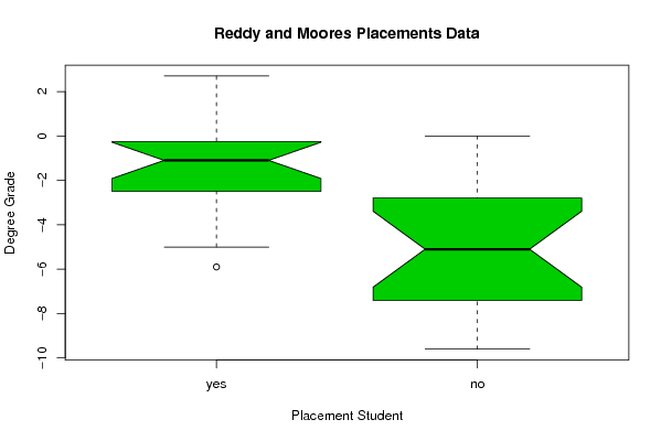
r<-boxplot(xtrm~as.factor(ytrm), col=par1, notch=par2, names =c('yes', 'no'), main='Reddy and Moores Placements Data', xlab='Placement Student', ylab='Degree Grade')
dev.off()
load(file='createtable')
a<-table.start()
a<-table.row.start(a)
a<-table.element(a,hyperlink('overview.htm','Boxplot statistics','Boxplot overview'),6,TRUE)
a<-table.row.end(a)
a<-table.row.start(a)
a<-table.element(a,'Placement',1,TRUE)
a<-table.element(a,hyperlink('lower_whisker.htm','lower whisker','definition of lower whisker'),1,TRUE)
a<-table.element(a,hyperlink('lower_hinge.htm','lower hinge','definition of lower hinge'),1,TRUE)
a<-table.element(a,hyperlink('central_tendency.htm','median','definitions about measures of central tendency'),1,TRUE)
a<-table.element(a,hyperlink('upper_hinge.htm','upper hinge','definition of upper hinge'),1,TRUE)
a<-table.element(a,hyperlink('upper_whisker.htm','upper whisker','definition of upper whisker'),1,TRUE)
a<-table.row.end(a)
a<-table.row.start(a)
a<-table.element(a,'yes',1,TRUE)
for (j in 1:5)
{
a<-table.element(a,r$stats[j,1])
}
a<-table.row.end(a)
a<-table.row.start(a)
a<-table.element(a,'no',1,TRUE)
for (j in 1:5)
{
a<-table.element(a,r$stats[j,2])
}
a<-table.row.end(a)
a<-table.end(a)
table.save(a,file='mytable.tab')
tr.mns<-tapply(x,y,mean, trim=par3/100)
a<-table.start()
a<-table.row.start(a)
a<-table.element(a,hyperlink('trimmed_mean.htm','Trimmed Mean Equation','Trimmed Mean'),2,TRUE)
a<-table.row.end(a)
a<-table.row.start(a)
a<-table.element(a,'Placement')
a<-table.element(a,'No Placement')
a<-table.row.end(a)
a<-table.row.start(a)
a<-table.element(a,tr.mns[1])
a<-table.element(a,tr.mns[2])
a<-table.row.end(a)
a<-table.end(a)
table.save(a,file='mytable1.tab')