Free Statistics
of Irreproducible Research!
Description of Statistical Computation | |||||||||||||||||||||||||||||||||
|---|---|---|---|---|---|---|---|---|---|---|---|---|---|---|---|---|---|---|---|---|---|---|---|---|---|---|---|---|---|---|---|---|---|
| Author's title | |||||||||||||||||||||||||||||||||
| Author | *Unverified author* | ||||||||||||||||||||||||||||||||
| R Software Module | rwasp_meanversusmedian.wasp | ||||||||||||||||||||||||||||||||
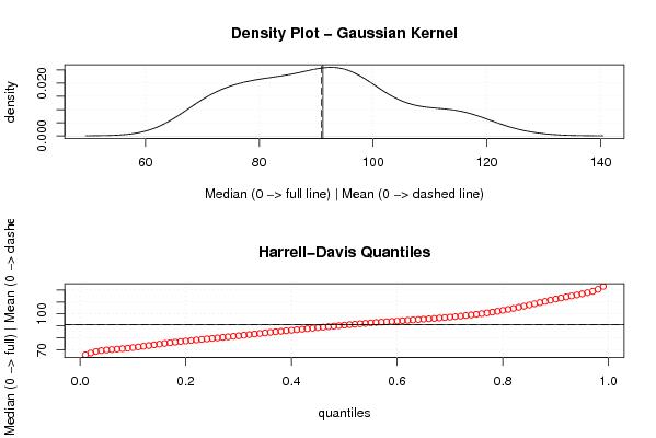
| Title produced by software | Mean versus Median | ||||||||||||||||||||||||||||||||
| Date of computation | Sun, 06 Jun 2010 19:39:14 +0000 | ||||||||||||||||||||||||||||||||
| Cite this page as follows | Statistical Computations at FreeStatistics.org, Office for Research Development and Education, URL https://freestatistics.org/blog/index.php?v=date/2010/Jun/06/t1275853232427hp1wvij5sf7u.htm/, Retrieved Sat, 27 Jul 2024 03:27:21 +0000 | ||||||||||||||||||||||||||||||||
| Statistical Computations at FreeStatistics.org, Office for Research Development and Education, URL https://freestatistics.org/blog/index.php?pk=77781, Retrieved Sat, 27 Jul 2024 03:27:21 +0000 | |||||||||||||||||||||||||||||||||
| QR Codes: | |||||||||||||||||||||||||||||||||
|
| |||||||||||||||||||||||||||||||||
| Original text written by user: | |||||||||||||||||||||||||||||||||
| IsPrivate? | No (this computation is public) | ||||||||||||||||||||||||||||||||
| User-defined keywords | KDGP1W52 | ||||||||||||||||||||||||||||||||
| Estimated Impact | 167 | ||||||||||||||||||||||||||||||||
Tree of Dependent Computations | |||||||||||||||||||||||||||||||||
| Family? (F = Feedback message, R = changed R code, M = changed R Module, P = changed Parameters, D = changed Data) | |||||||||||||||||||||||||||||||||
| - [Notched Boxplots] [Opgave 3 - box pl...] [2010-03-03 16:55:40] [74be16979710d4c4e7c6647856088456] - RM D [Mean versus Median] [mediaan - rekenku...] [2010-06-06 19:39:14] [0291ee60c135beb64d296f3dc8feb2dc] [Current] | |||||||||||||||||||||||||||||||||
| Feedback Forum | |||||||||||||||||||||||||||||||||
Post a new message | |||||||||||||||||||||||||||||||||
Dataset | |||||||||||||||||||||||||||||||||
| Dataseries X: | |||||||||||||||||||||||||||||||||
93.2 96 95.2 77.1 70.9 64.8 70.1 77.3 79.5 100.6 100.7 107.1 95.9 82.8 83.3 80 80.4 67.5 75.7 71.1 89.3 101.1 105.2 114.1 96.3 84.4 91.2 81.9 80.5 70.4 74.8 75.9 86.3 98.7 100.9 113.8 89.8 84.4 87.2 85.6 72 69.2 77.5 78.1 94.3 97.7 100.2 116.4 97.1 93 96 80.5 76.1 69.9 73.6 92.6 94.2 93.5 108.5 109.4 105.1 92.5 97.1 81.4 79.1 72.1 78.7 87.1 91.4 109.9 116.3 113 100 84.8 94.3 87.1 90.3 72.4 84.9 92.7 92.2 114.9 112.5 118.3 106 91.2 96.6 96.3 88.2 70.2 86.5 88.2 102.8 119.1 119.2 125.1 | |||||||||||||||||||||||||||||||||
Tables (Output of Computation) | |||||||||||||||||||||||||||||||||
| |||||||||||||||||||||||||||||||||
Figures (Output of Computation) | |||||||||||||||||||||||||||||||||
Input Parameters & R Code | |||||||||||||||||||||||||||||||||
| Parameters (Session): | |||||||||||||||||||||||||||||||||
| par1 = grey ; | |||||||||||||||||||||||||||||||||
| Parameters (R input): | |||||||||||||||||||||||||||||||||
| R code (references can be found in the software module): | |||||||||||||||||||||||||||||||||
library(Hmisc) | |||||||||||||||||||||||||||||||||