Free Statistics
of Irreproducible Research!
Description of Statistical Computation | |||||||||||||||||||||||||||||||||||||||||||||||||||||||||||||||||||||||||||||||||
|---|---|---|---|---|---|---|---|---|---|---|---|---|---|---|---|---|---|---|---|---|---|---|---|---|---|---|---|---|---|---|---|---|---|---|---|---|---|---|---|---|---|---|---|---|---|---|---|---|---|---|---|---|---|---|---|---|---|---|---|---|---|---|---|---|---|---|---|---|---|---|---|---|---|---|---|---|---|---|---|---|---|
| Author's title | |||||||||||||||||||||||||||||||||||||||||||||||||||||||||||||||||||||||||||||||||
| Author | *The author of this computation has been verified* | ||||||||||||||||||||||||||||||||||||||||||||||||||||||||||||||||||||||||||||||||
| R Software Module | Ian.Hollidayrwasp_Reddy-Moores Data Boxplot.wasp | ||||||||||||||||||||||||||||||||||||||||||||||||||||||||||||||||||||||||||||||||
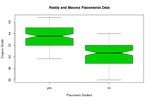
| Title produced by software | Boxplot and Trimmed Means | ||||||||||||||||||||||||||||||||||||||||||||||||||||||||||||||||||||||||||||||||
| Date of computation | Wed, 05 May 2010 15:58:40 +0000 | ||||||||||||||||||||||||||||||||||||||||||||||||||||||||||||||||||||||||||||||||
| Cite this page as follows | Statistical Computations at FreeStatistics.org, Office for Research Development and Education, URL https://freestatistics.org/blog/index.php?v=date/2010/May/05/t1273075184f010grgah5rra8r.htm/, Retrieved Sat, 27 Apr 2024 17:21:21 +0000 | ||||||||||||||||||||||||||||||||||||||||||||||||||||||||||||||||||||||||||||||||
| Statistical Computations at FreeStatistics.org, Office for Research Development and Education, URL https://freestatistics.org/blog/index.php?pk=75547, Retrieved Sat, 27 Apr 2024 17:21:21 +0000 | |||||||||||||||||||||||||||||||||||||||||||||||||||||||||||||||||||||||||||||||||
| QR Codes: | |||||||||||||||||||||||||||||||||||||||||||||||||||||||||||||||||||||||||||||||||
|
| |||||||||||||||||||||||||||||||||||||||||||||||||||||||||||||||||||||||||||||||||
| Original text written by user: | |||||||||||||||||||||||||||||||||||||||||||||||||||||||||||||||||||||||||||||||||
| IsPrivate? | No (this computation is public) | ||||||||||||||||||||||||||||||||||||||||||||||||||||||||||||||||||||||||||||||||
| User-defined keywords | boxplots, Reddy-Moores placement data, Aston Unviversity | ||||||||||||||||||||||||||||||||||||||||||||||||||||||||||||||||||||||||||||||||
| Estimated Impact | 148 | ||||||||||||||||||||||||||||||||||||||||||||||||||||||||||||||||||||||||||||||||
Tree of Dependent Computations | |||||||||||||||||||||||||||||||||||||||||||||||||||||||||||||||||||||||||||||||||
| Family? (F = Feedback message, R = changed R code, M = changed R Module, P = changed Parameters, D = changed Data) | |||||||||||||||||||||||||||||||||||||||||||||||||||||||||||||||||||||||||||||||||
| - [Boxplot and Trimmed Means] [Reddy-Moores Plac...] [2010-05-05 15:58:40] [a9208f4f8d3b118336aae915785f2bd9] [Current] | |||||||||||||||||||||||||||||||||||||||||||||||||||||||||||||||||||||||||||||||||
| Feedback Forum | |||||||||||||||||||||||||||||||||||||||||||||||||||||||||||||||||||||||||||||||||
Post a new message | |||||||||||||||||||||||||||||||||||||||||||||||||||||||||||||||||||||||||||||||||
Dataset | |||||||||||||||||||||||||||||||||||||||||||||||||||||||||||||||||||||||||||||||||
| Dataseries X: | |||||||||||||||||||||||||||||||||||||||||||||||||||||||||||||||||||||||||||||||||
70.80 69.60 69.87 67.47 67.60 67.13 66.27 66.73 68.07 67.80 64.80 64.60 64.20 64.20 63.67 61.00 59.67 59.67 59.80 60.73 59.40 58.07 57.47 66.67 66.33 64.33 64.00 63.33 61.33 64.67 63.00 60.67 63.67 60.67 61.67 62.33 60.33 59.67 60.33 59.33 58.67 58.67 59.33 57.33 59.33 56.00 53.67 58.67 49.33 70.73 72.87 66.00 66.07 66.00 66.27 64.00 63.67 63.73 63.33 63.53 63.53 62.87 59.53 62.80 60.80 59.80 56.67 57.67 58.40 55.47 56.20 71.33 70.33 69.00 66.00 66.00 63.33 65.33 64.33 64.00 61.67 63.67 64.67 61.67 62.00 61.33 63.67 61.33 62.33 59.67 59.33 61.67 58.67 58.00 56.67 59.67 58.00 57.00 57.67 58.67 55.33 56.00 55.67 53.33 53.67 51.00 47.00 4.33 71.53 68.67 65.67 66.73 67.33 66.73 66.87 65.80 64.73 65.47 63.60 64.07 64.67 63.73 62.53 61.93 62.67 62.80 61.33 62.60 59.13 61.27 59.47 57.87 59.73 61.40 58.80 58.33 57.47 57.13 55.00 51.53 70.00 68.67 67.67 66.00 65.67 65.67 63.67 63.67 64.00 62.00 62.00 61.67 61.67 63.33 61.00 62.33 60.33 60.33 60.67 57.67 58.33 58.00 57.33 56.67 58.00 55.33 55.67 54.67 56.33 55.00 55.00 54.67 54.33 49.00 48.33 49.67 43.67 6.33 3.00 72.73 73.00 70.80 70.07 71.67 71.07 70.67 70.73 70.73 68.60 69.60 66.47 67.07 68.67 66.93 65.93 68.87 66.53 65.80 66.60 66.00 65.00 66.80 65.60 66.00 65.67 64.67 65.07 64.67 65.07 65.20 64.87 63.47 62.60 64.07 63.73 64.67 61.60 61.60 60.47 61.27 63.00 61.47 60.87 61.67 62.87 62.40 59.73 60.13 58.80 59.60 58.93 60.13 58.20 58.27 58.27 55.07 53.87 52.33 47.20 37.93 66.67 67.33 65.33 66.00 65.67 66.67 65.67 65.00 64.67 66.67 63.67 63.33 63.67 63.33 63.67 63.00 61.67 61.33 60.67 60.00 61.67 61.33 58.67 60.33 59.67 59.33 59.67 61.00 61.00 60.00 60.00 58.67 58.33 58.00 56.33 54.67 55.33 54.00 52.67 44.00 72.73 70.07 70.67 72.07 68.80 68.80 67.47 66.73 66.53 66.00 67.60 66.00 66.00 66.53 65.80 64.27 64.67 64.60 64.13 65.47 62.93 63.53 62.13 63.87 64.67 63.33 63.13 62.80 62.40 62.40 62.60 61.47 62.20 63.00 61.80 59.73 60.33 60.13 59.53 59.00 55.93 41.87 36.33 65.67 65.00 66.33 64.00 62.33 61.33 63.00 63.67 62.00 61.33 64.67 62.67 64.00 61.00 60.67 59.67 60.33 56.67 56.67 54.33 51.00 51.00 47.00 71.67 71.47 70.47 69.53 70.73 69.93 68.73 67.53 64.40 66.20 66.20 63.07 64.27 65.00 63.67 62.67 64.67 64.67 64.47 61.93 63.27 62.93 61.93 64.07 61.40 62.00 62.60 62.40 61.60 59.87 63.20 62.40 60.40 61.87 59.13 59.53 57.80 57.67 61.00 56.33 54.20 54.73 52.67 17.60 68 65 64 64 64 62 61 60 60 62 60 59 61 60 60 58 58 60 58 59 56 54 51 47 | |||||||||||||||||||||||||||||||||||||||||||||||||||||||||||||||||||||||||||||||||
| Dataseries Y: | |||||||||||||||||||||||||||||||||||||||||||||||||||||||||||||||||||||||||||||||||
1 1 1 1 1 1 1 1 1 1 1 1 1 1 1 1 1 1 1 1 1 1 1 2 2 2 2 2 2 2 2 2 2 2 2 2 2 2 2 2 2 2 2 2 2 2 2 2 2 1 1 1 1 1 1 1 1 1 1 1 1 1 1 1 1 1 1 1 1 1 1 2 2 2 2 2 2 2 2 2 2 2 2 2 2 2 2 2 2 2 2 2 2 2 2 2 2 2 2 2 2 2 2 2 2 2 2 2 1 1 1 1 1 1 1 1 1 1 1 1 1 1 1 1 1 1 1 1 1 1 1 1 1 1 1 1 1 1 1 1 2 2 2 2 2 2 2 2 2 2 2 2 2 2 2 2 2 2 2 2 2 2 2 2 2 2 2 2 2 2 2 2 2 2 2 2 2 2 2 1 1 1 1 1 1 1 1 1 1 1 1 1 1 1 1 1 1 1 1 1 1 1 1 1 1 1 1 1 1 1 1 1 1 1 1 1 1 1 1 1 1 1 1 1 1 1 1 1 1 1 1 1 1 1 1 1 1 1 1 1 2 2 2 2 2 2 2 2 2 2 2 2 2 2 2 2 2 2 2 2 2 2 2 2 2 2 2 2 2 2 2 2 2 2 2 2 2 2 2 2 1 1 1 1 1 1 1 1 1 1 1 1 1 1 1 1 1 1 1 1 1 1 1 1 1 1 1 1 1 1 1 1 1 1 1 1 1 1 1 1 1 1 1 2 2 2 2 2 2 2 2 2 2 2 2 2 2 2 2 2 2 2 2 2 2 2 1 1 1 1 1 1 1 1 1 1 1 1 1 1 1 1 1 1 1 1 1 1 1 1 1 1 1 1 1 1 1 1 1 1 1 1 1 1 1 1 1 1 1 1 2 2 2 2 2 2 2 2 2 2 2 2 2 2 2 2 2 2 2 2 2 2 2 2 | |||||||||||||||||||||||||||||||||||||||||||||||||||||||||||||||||||||||||||||||||
Tables (Output of Computation) | |||||||||||||||||||||||||||||||||||||||||||||||||||||||||||||||||||||||||||||||||
| |||||||||||||||||||||||||||||||||||||||||||||||||||||||||||||||||||||||||||||||||
Figures (Output of Computation) | |||||||||||||||||||||||||||||||||||||||||||||||||||||||||||||||||||||||||||||||||
Input Parameters & R Code | |||||||||||||||||||||||||||||||||||||||||||||||||||||||||||||||||||||||||||||||||
| Parameters (Session): | |||||||||||||||||||||||||||||||||||||||||||||||||||||||||||||||||||||||||||||||||
| par1 = 3 ; par2 = TRUE ; par3 = 20 ; | |||||||||||||||||||||||||||||||||||||||||||||||||||||||||||||||||||||||||||||||||
| Parameters (R input): | |||||||||||||||||||||||||||||||||||||||||||||||||||||||||||||||||||||||||||||||||
| par1 = 3 ; par2 = TRUE ; par3 = 20 ; | |||||||||||||||||||||||||||||||||||||||||||||||||||||||||||||||||||||||||||||||||
| R code (references can be found in the software module): | |||||||||||||||||||||||||||||||||||||||||||||||||||||||||||||||||||||||||||||||||
bitmap(file='test1.png') | |||||||||||||||||||||||||||||||||||||||||||||||||||||||||||||||||||||||||||||||||