Repository of Reproducible Computations

Free Statistics

of Irreproducible Research!

Author's title

Author

*Unverified author*

R Software Module

rwasp_autocorrelation.wasp

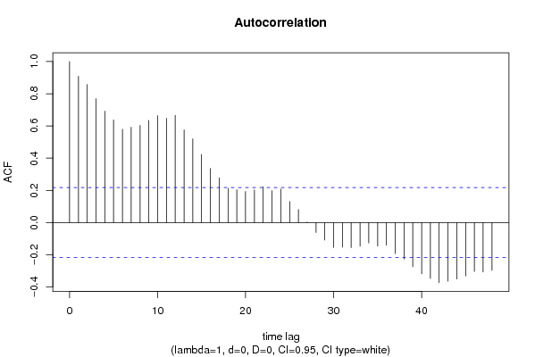
Title produced by software

(Partial) Autocorrelation Function

Date of computation

Wed, 05 May 2010 19:31:00 +0000

Cite this page as follows

Statistical Computations at FreeStatistics.org, Office for Research Development and Education, URL https://freestatistics.org/blog/index.php?v=date/2010/May/05/t1273087893z3pw9npm7c6n69r.htm/, Retrieved Sat, 27 Apr 2024 18:22:13 +0000

Statistical Computations at FreeStatistics.org, Office for Research Development and Education, URL https://freestatistics.org/blog/index.php?pk=75574, Retrieved Sat, 27 Apr 2024 18:22:13 +0000

QR Codes:

Paste this QR Code to cite your computation.

Original text written by user:

IsPrivate?

No (this computation is public)

User-defined keywords

KDGP2W21

Estimated Impact

122

Family? (F = Feedback message, R = changed R code, M = changed R Module, P = changed Parameters, D = changed Data)

-       [(Partial) Autocorrelation Function] [Energieverbruik ] [2010-05-05 19:31:00] [dd2ef098fd65ce7e9f689caa343b799f] [Current]

Feedback Forum

Post a new message

Dataseries X:

Download CSV

Histogram

Boxplots

Summary of computational transaction
Raw Input	view raw input (R code)
Raw Output	view raw output of R engine
Computing time	1 seconds
R Server	'Gwilym Jenkins' @ 72.249.127.135

\begin{tabular}{lllllllll}
\hline
Summary of computational transaction \tabularnewline
Raw Input & view raw input (R code)  \tabularnewline
Raw Output & view raw output of R engine  \tabularnewline
Computing time & 1 seconds \tabularnewline
R Server & 'Gwilym Jenkins' @ 72.249.127.135 \tabularnewline
\hline
\end{tabular}
%Source: https://freestatistics.org/blog/index.php?pk=75574&T=0

[TABLE]
[ROW][C]Summary of computational transaction[/C][/ROW]
[ROW][C]Raw Input[/C][C]view raw input (R code) [/C][/ROW]
[ROW][C]Raw Output[/C][C]view raw output of R engine [/C][/ROW]
[ROW][C]Computing time[/C][C]1 seconds[/C][/ROW]
[ROW][C]R Server[/C][C]'Gwilym Jenkins' @ 72.249.127.135[/C][/ROW]
[/TABLE]
Source: https://freestatistics.org/blog/index.php?pk=75574&T=0

Globally Unique Identifier (entire table): ba.freestatistics.org/blog/index.php?pk=75574&T=0

As an alternative you can also use a QR Code:

The GUIDs for individual cells are displayed in the table below:

Summary of computational transaction
Raw Input	view raw input (R code)
Raw Output	view raw output of R engine
Computing time	1 seconds
R Server	'Gwilym Jenkins' @ 72.249.127.135

Autocorrelation Function
Time lag k	ACF(k)	T-STAT	P-value
1	0.908729	8.1786	0
2	0.857339	7.716	0
3	0.769587	6.9263	0
4	0.691766	6.2259	0
5	0.637726	5.7395	0
6	0.579896	5.2191	1e-06
7	0.592171	5.3295	0
8	0.603238	5.4291	0
9	0.634653	5.7119	0
10	0.664381	5.9794	0
11	0.647506	5.8276	0
12	0.66652	5.9987	0
13	0.575598	5.1804	1e-06
14	0.520029	4.6803	6e-06
15	0.42341	3.8107	0.000134
16	0.336927	3.0323	0.00163
17	0.277937	2.5014	0.007192
18	0.212431	1.9119	0.029714
19	0.204035	1.8363	0.03499
20	0.193464	1.7412	0.042725
21	0.202727	1.8245	0.035879
22	0.223374	2.0104	0.02386
23	0.198014	1.7821	0.039238
24	0.208175	1.8736	0.032298
25	0.130764	1.1769	0.121346
26	0.081474	0.7333	0.232757
27	0.003617	0.0326	0.487056
28	-0.061152	-0.5504	0.291791
29	-0.108118	-0.9731	0.166709
30	-0.1537	-1.3833	0.085187
31	-0.152072	-1.3686	0.087447
32	-0.15502	-1.3952	0.083388
33	-0.146107	-1.315	0.096117
34	-0.125748	-1.1317	0.130542
35	-0.145118	-1.3061	0.097615
36	-0.140254	-1.2623	0.105235
37	-0.192811	-1.7353	0.043245
38	-0.22629	-2.0366	0.022478
39	-0.274162	-2.4675	0.007858
40	-0.318094	-2.8628	0.002671
41	-0.346359	-3.1172	0.001263
42	-0.37241	-3.3517	0.000611
43	-0.363612	-3.2725	0.000784
44	-0.350445	-3.154	0.00113
45	-0.330971	-2.9787	0.001909
46	-0.303012	-2.7271	0.003915
47	-0.307089	-2.7638	0.003535
48	-0.296361	-2.6672	0.004616

\begin{tabular}{lllllllll}
\hline
Autocorrelation Function \tabularnewline
Time lag k & ACF(k) & T-STAT & P-value \tabularnewline
1 & 0.908729 & 8.1786 & 0 \tabularnewline
2 & 0.857339 & 7.716 & 0 \tabularnewline
3 & 0.769587 & 6.9263 & 0 \tabularnewline
4 & 0.691766 & 6.2259 & 0 \tabularnewline
5 & 0.637726 & 5.7395 & 0 \tabularnewline
6 & 0.579896 & 5.2191 & 1e-06 \tabularnewline
7 & 0.592171 & 5.3295 & 0 \tabularnewline
8 & 0.603238 & 5.4291 & 0 \tabularnewline
9 & 0.634653 & 5.7119 & 0 \tabularnewline
10 & 0.664381 & 5.9794 & 0 \tabularnewline
11 & 0.647506 & 5.8276 & 0 \tabularnewline
12 & 0.66652 & 5.9987 & 0 \tabularnewline
13 & 0.575598 & 5.1804 & 1e-06 \tabularnewline
14 & 0.520029 & 4.6803 & 6e-06 \tabularnewline
15 & 0.42341 & 3.8107 & 0.000134 \tabularnewline
16 & 0.336927 & 3.0323 & 0.00163 \tabularnewline
17 & 0.277937 & 2.5014 & 0.007192 \tabularnewline
18 & 0.212431 & 1.9119 & 0.029714 \tabularnewline
19 & 0.204035 & 1.8363 & 0.03499 \tabularnewline
20 & 0.193464 & 1.7412 & 0.042725 \tabularnewline
21 & 0.202727 & 1.8245 & 0.035879 \tabularnewline
22 & 0.223374 & 2.0104 & 0.02386 \tabularnewline
23 & 0.198014 & 1.7821 & 0.039238 \tabularnewline
24 & 0.208175 & 1.8736 & 0.032298 \tabularnewline
25 & 0.130764 & 1.1769 & 0.121346 \tabularnewline
26 & 0.081474 & 0.7333 & 0.232757 \tabularnewline
27 & 0.003617 & 0.0326 & 0.487056 \tabularnewline
28 & -0.061152 & -0.5504 & 0.291791 \tabularnewline
29 & -0.108118 & -0.9731 & 0.166709 \tabularnewline
30 & -0.1537 & -1.3833 & 0.085187 \tabularnewline
31 & -0.152072 & -1.3686 & 0.087447 \tabularnewline
32 & -0.15502 & -1.3952 & 0.083388 \tabularnewline
33 & -0.146107 & -1.315 & 0.096117 \tabularnewline
34 & -0.125748 & -1.1317 & 0.130542 \tabularnewline
35 & -0.145118 & -1.3061 & 0.097615 \tabularnewline
36 & -0.140254 & -1.2623 & 0.105235 \tabularnewline
37 & -0.192811 & -1.7353 & 0.043245 \tabularnewline
38 & -0.22629 & -2.0366 & 0.022478 \tabularnewline
39 & -0.274162 & -2.4675 & 0.007858 \tabularnewline
40 & -0.318094 & -2.8628 & 0.002671 \tabularnewline
41 & -0.346359 & -3.1172 & 0.001263 \tabularnewline
42 & -0.37241 & -3.3517 & 0.000611 \tabularnewline
43 & -0.363612 & -3.2725 & 0.000784 \tabularnewline
44 & -0.350445 & -3.154 & 0.00113 \tabularnewline
45 & -0.330971 & -2.9787 & 0.001909 \tabularnewline
46 & -0.303012 & -2.7271 & 0.003915 \tabularnewline
47 & -0.307089 & -2.7638 & 0.003535 \tabularnewline
48 & -0.296361 & -2.6672 & 0.004616 \tabularnewline
\hline
\end{tabular}
%Source: https://freestatistics.org/blog/index.php?pk=75574&T=1

[TABLE]
[ROW][C]Autocorrelation Function[/C][/ROW]
[ROW][C]Time lag k[/C][C]ACF(k)[/C][C]T-STAT[/C][C]P-value[/C][/ROW]
[ROW][C]1[/C][C]0.908729[/C][C]8.1786[/C][C]0[/C][/ROW]
[ROW][C]2[/C][C]0.857339[/C][C]7.716[/C][C]0[/C][/ROW]
[ROW][C]3[/C][C]0.769587[/C][C]6.9263[/C][C]0[/C][/ROW]
[ROW][C]4[/C][C]0.691766[/C][C]6.2259[/C][C]0[/C][/ROW]
[ROW][C]5[/C][C]0.637726[/C][C]5.7395[/C][C]0[/C][/ROW]
[ROW][C]6[/C][C]0.579896[/C][C]5.2191[/C][C]1e-06[/C][/ROW]
[ROW][C]7[/C][C]0.592171[/C][C]5.3295[/C][C]0[/C][/ROW]
[ROW][C]8[/C][C]0.603238[/C][C]5.4291[/C][C]0[/C][/ROW]
[ROW][C]9[/C][C]0.634653[/C][C]5.7119[/C][C]0[/C][/ROW]
[ROW][C]10[/C][C]0.664381[/C][C]5.9794[/C][C]0[/C][/ROW]
[ROW][C]11[/C][C]0.647506[/C][C]5.8276[/C][C]0[/C][/ROW]
[ROW][C]12[/C][C]0.66652[/C][C]5.9987[/C][C]0[/C][/ROW]
[ROW][C]13[/C][C]0.575598[/C][C]5.1804[/C][C]1e-06[/C][/ROW]
[ROW][C]14[/C][C]0.520029[/C][C]4.6803[/C][C]6e-06[/C][/ROW]
[ROW][C]15[/C][C]0.42341[/C][C]3.8107[/C][C]0.000134[/C][/ROW]
[ROW][C]16[/C][C]0.336927[/C][C]3.0323[/C][C]0.00163[/C][/ROW]
[ROW][C]17[/C][C]0.277937[/C][C]2.5014[/C][C]0.007192[/C][/ROW]
[ROW][C]18[/C][C]0.212431[/C][C]1.9119[/C][C]0.029714[/C][/ROW]
[ROW][C]19[/C][C]0.204035[/C][C]1.8363[/C][C]0.03499[/C][/ROW]
[ROW][C]20[/C][C]0.193464[/C][C]1.7412[/C][C]0.042725[/C][/ROW]
[ROW][C]21[/C][C]0.202727[/C][C]1.8245[/C][C]0.035879[/C][/ROW]
[ROW][C]22[/C][C]0.223374[/C][C]2.0104[/C][C]0.02386[/C][/ROW]
[ROW][C]23[/C][C]0.198014[/C][C]1.7821[/C][C]0.039238[/C][/ROW]
[ROW][C]24[/C][C]0.208175[/C][C]1.8736[/C][C]0.032298[/C][/ROW]
[ROW][C]25[/C][C]0.130764[/C][C]1.1769[/C][C]0.121346[/C][/ROW]
[ROW][C]26[/C][C]0.081474[/C][C]0.7333[/C][C]0.232757[/C][/ROW]
[ROW][C]27[/C][C]0.003617[/C][C]0.0326[/C][C]0.487056[/C][/ROW]
[ROW][C]28[/C][C]-0.061152[/C][C]-0.5504[/C][C]0.291791[/C][/ROW]
[ROW][C]29[/C][C]-0.108118[/C][C]-0.9731[/C][C]0.166709[/C][/ROW]
[ROW][C]30[/C][C]-0.1537[/C][C]-1.3833[/C][C]0.085187[/C][/ROW]
[ROW][C]31[/C][C]-0.152072[/C][C]-1.3686[/C][C]0.087447[/C][/ROW]
[ROW][C]32[/C][C]-0.15502[/C][C]-1.3952[/C][C]0.083388[/C][/ROW]
[ROW][C]33[/C][C]-0.146107[/C][C]-1.315[/C][C]0.096117[/C][/ROW]
[ROW][C]34[/C][C]-0.125748[/C][C]-1.1317[/C][C]0.130542[/C][/ROW]
[ROW][C]35[/C][C]-0.145118[/C][C]-1.3061[/C][C]0.097615[/C][/ROW]
[ROW][C]36[/C][C]-0.140254[/C][C]-1.2623[/C][C]0.105235[/C][/ROW]
[ROW][C]37[/C][C]-0.192811[/C][C]-1.7353[/C][C]0.043245[/C][/ROW]
[ROW][C]38[/C][C]-0.22629[/C][C]-2.0366[/C][C]0.022478[/C][/ROW]
[ROW][C]39[/C][C]-0.274162[/C][C]-2.4675[/C][C]0.007858[/C][/ROW]
[ROW][C]40[/C][C]-0.318094[/C][C]-2.8628[/C][C]0.002671[/C][/ROW]
[ROW][C]41[/C][C]-0.346359[/C][C]-3.1172[/C][C]0.001263[/C][/ROW]
[ROW][C]42[/C][C]-0.37241[/C][C]-3.3517[/C][C]0.000611[/C][/ROW]
[ROW][C]43[/C][C]-0.363612[/C][C]-3.2725[/C][C]0.000784[/C][/ROW]
[ROW][C]44[/C][C]-0.350445[/C][C]-3.154[/C][C]0.00113[/C][/ROW]
[ROW][C]45[/C][C]-0.330971[/C][C]-2.9787[/C][C]0.001909[/C][/ROW]
[ROW][C]46[/C][C]-0.303012[/C][C]-2.7271[/C][C]0.003915[/C][/ROW]
[ROW][C]47[/C][C]-0.307089[/C][C]-2.7638[/C][C]0.003535[/C][/ROW]
[ROW][C]48[/C][C]-0.296361[/C][C]-2.6672[/C][C]0.004616[/C][/ROW]
[/TABLE]
Source: https://freestatistics.org/blog/index.php?pk=75574&T=1

Globally Unique Identifier (entire table): ba.freestatistics.org/blog/index.php?pk=75574&T=1

As an alternative you can also use a QR Code:

The GUIDs for individual cells are displayed in the table below:

Autocorrelation Function
Time lag k	ACF(k)	T-STAT	P-value
1	0.908729	8.1786	0
2	0.857339	7.716	0
3	0.769587	6.9263	0
4	0.691766	6.2259	0
5	0.637726	5.7395	0
6	0.579896	5.2191	1e-06
7	0.592171	5.3295	0
8	0.603238	5.4291	0
9	0.634653	5.7119	0
10	0.664381	5.9794	0
11	0.647506	5.8276	0
12	0.66652	5.9987	0
13	0.575598	5.1804	1e-06
14	0.520029	4.6803	6e-06
15	0.42341	3.8107	0.000134
16	0.336927	3.0323	0.00163
17	0.277937	2.5014	0.007192
18	0.212431	1.9119	0.029714
19	0.204035	1.8363	0.03499
20	0.193464	1.7412	0.042725
21	0.202727	1.8245	0.035879
22	0.223374	2.0104	0.02386
23	0.198014	1.7821	0.039238
24	0.208175	1.8736	0.032298
25	0.130764	1.1769	0.121346
26	0.081474	0.7333	0.232757
27	0.003617	0.0326	0.487056
28	-0.061152	-0.5504	0.291791
29	-0.108118	-0.9731	0.166709
30	-0.1537	-1.3833	0.085187
31	-0.152072	-1.3686	0.087447
32	-0.15502	-1.3952	0.083388
33	-0.146107	-1.315	0.096117
34	-0.125748	-1.1317	0.130542
35	-0.145118	-1.3061	0.097615
36	-0.140254	-1.2623	0.105235
37	-0.192811	-1.7353	0.043245
38	-0.22629	-2.0366	0.022478
39	-0.274162	-2.4675	0.007858
40	-0.318094	-2.8628	0.002671
41	-0.346359	-3.1172	0.001263
42	-0.37241	-3.3517	0.000611
43	-0.363612	-3.2725	0.000784
44	-0.350445	-3.154	0.00113
45	-0.330971	-2.9787	0.001909
46	-0.303012	-2.7271	0.003915
47	-0.307089	-2.7638	0.003535
48	-0.296361	-2.6672	0.004616

Partial Autocorrelation Function
Time lag k	PACF(k)	T-STAT	P-value
1	0.908729	8.1786	0
2	0.181107	1.63	0.053497
3	-0.195727	-1.7615	0.04096
4	-0.064689	-0.5822	0.281024
5	0.141301	1.2717	0.103558
6	-0.001767	-0.0159	0.493676
7	0.341122	3.0701	0.001456
8	0.167055	1.5035	0.0683
9	0.053807	0.4843	0.314753
10	0.04562	0.4106	0.341234
11	-0.223383	-2.0104	0.023856
12	0.174177	1.5676	0.060437
13	-0.450638	-4.0557	5.7e-05
14	0.006324	0.0569	0.477377
15	-0.140912	-1.2682	0.104178
16	-0.09897	-0.8907	0.187857
17	-0.04213	-0.3792	0.352776
18	-0.05277	-0.4749	0.318058
19	-0.034074	-0.3067	0.379943
20	0.012422	0.1118	0.455632
21	-0.012794	-0.1152	0.454305
22	0.089821	0.8084	0.210617
23	-0.041033	-0.3693	0.356435
24	0.060196	0.5418	0.294733
25	-0.100142	-0.9013	0.185056
26	-0.044887	-0.404	0.343646
27	0.038884	0.35	0.363639
28	0.059324	0.5339	0.297431
29	-0.082812	-0.7453	0.229122
30	0.065608	0.5905	0.278259
31	-0.034263	-0.3084	0.379298
32	-0.039636	-0.3567	0.361111
33	-0.037733	-0.3396	0.367519
34	-0.007293	-0.0656	0.473913
35	-0.00674	-0.0607	0.475888
36	-0.092953	-0.8366	0.202645
37	0.047428	0.4269	0.335309
38	-0.05874	-0.5287	0.299242
39	0.048234	0.4341	0.332684
40	-0.064634	-0.5817	0.281191
41	-0.027592	-0.2483	0.402255
42	-0.019014	-0.1711	0.432274
43	0.00629	0.0566	0.477497
44	0.047713	0.4294	0.334381
45	0.031745	0.2857	0.387916
46	-0.046508	-0.4186	0.338319
47	0.00477	0.0429	0.482933
48	-0.0619	-0.5571	0.289499

\begin{tabular}{lllllllll}
\hline
Partial Autocorrelation Function \tabularnewline
Time lag k & PACF(k) & T-STAT & P-value \tabularnewline
1 & 0.908729 & 8.1786 & 0 \tabularnewline
2 & 0.181107 & 1.63 & 0.053497 \tabularnewline
3 & -0.195727 & -1.7615 & 0.04096 \tabularnewline
4 & -0.064689 & -0.5822 & 0.281024 \tabularnewline
5 & 0.141301 & 1.2717 & 0.103558 \tabularnewline
6 & -0.001767 & -0.0159 & 0.493676 \tabularnewline
7 & 0.341122 & 3.0701 & 0.001456 \tabularnewline
8 & 0.167055 & 1.5035 & 0.0683 \tabularnewline
9 & 0.053807 & 0.4843 & 0.314753 \tabularnewline
10 & 0.04562 & 0.4106 & 0.341234 \tabularnewline
11 & -0.223383 & -2.0104 & 0.023856 \tabularnewline
12 & 0.174177 & 1.5676 & 0.060437 \tabularnewline
13 & -0.450638 & -4.0557 & 5.7e-05 \tabularnewline
14 & 0.006324 & 0.0569 & 0.477377 \tabularnewline
15 & -0.140912 & -1.2682 & 0.104178 \tabularnewline
16 & -0.09897 & -0.8907 & 0.187857 \tabularnewline
17 & -0.04213 & -0.3792 & 0.352776 \tabularnewline
18 & -0.05277 & -0.4749 & 0.318058 \tabularnewline
19 & -0.034074 & -0.3067 & 0.379943 \tabularnewline
20 & 0.012422 & 0.1118 & 0.455632 \tabularnewline
21 & -0.012794 & -0.1152 & 0.454305 \tabularnewline
22 & 0.089821 & 0.8084 & 0.210617 \tabularnewline
23 & -0.041033 & -0.3693 & 0.356435 \tabularnewline
24 & 0.060196 & 0.5418 & 0.294733 \tabularnewline
25 & -0.100142 & -0.9013 & 0.185056 \tabularnewline
26 & -0.044887 & -0.404 & 0.343646 \tabularnewline
27 & 0.038884 & 0.35 & 0.363639 \tabularnewline
28 & 0.059324 & 0.5339 & 0.297431 \tabularnewline
29 & -0.082812 & -0.7453 & 0.229122 \tabularnewline
30 & 0.065608 & 0.5905 & 0.278259 \tabularnewline
31 & -0.034263 & -0.3084 & 0.379298 \tabularnewline
32 & -0.039636 & -0.3567 & 0.361111 \tabularnewline
33 & -0.037733 & -0.3396 & 0.367519 \tabularnewline
34 & -0.007293 & -0.0656 & 0.473913 \tabularnewline
35 & -0.00674 & -0.0607 & 0.475888 \tabularnewline
36 & -0.092953 & -0.8366 & 0.202645 \tabularnewline
37 & 0.047428 & 0.4269 & 0.335309 \tabularnewline
38 & -0.05874 & -0.5287 & 0.299242 \tabularnewline
39 & 0.048234 & 0.4341 & 0.332684 \tabularnewline
40 & -0.064634 & -0.5817 & 0.281191 \tabularnewline
41 & -0.027592 & -0.2483 & 0.402255 \tabularnewline
42 & -0.019014 & -0.1711 & 0.432274 \tabularnewline
43 & 0.00629 & 0.0566 & 0.477497 \tabularnewline
44 & 0.047713 & 0.4294 & 0.334381 \tabularnewline
45 & 0.031745 & 0.2857 & 0.387916 \tabularnewline
46 & -0.046508 & -0.4186 & 0.338319 \tabularnewline
47 & 0.00477 & 0.0429 & 0.482933 \tabularnewline
48 & -0.0619 & -0.5571 & 0.289499 \tabularnewline
\hline
\end{tabular}
%Source: https://freestatistics.org/blog/index.php?pk=75574&T=2

[TABLE]
[ROW][C]Partial Autocorrelation Function[/C][/ROW]
[ROW][C]Time lag k[/C][C]PACF(k)[/C][C]T-STAT[/C][C]P-value[/C][/ROW]
[ROW][C]1[/C][C]0.908729[/C][C]8.1786[/C][C]0[/C][/ROW]
[ROW][C]2[/C][C]0.181107[/C][C]1.63[/C][C]0.053497[/C][/ROW]
[ROW][C]3[/C][C]-0.195727[/C][C]-1.7615[/C][C]0.04096[/C][/ROW]
[ROW][C]4[/C][C]-0.064689[/C][C]-0.5822[/C][C]0.281024[/C][/ROW]
[ROW][C]5[/C][C]0.141301[/C][C]1.2717[/C][C]0.103558[/C][/ROW]
[ROW][C]6[/C][C]-0.001767[/C][C]-0.0159[/C][C]0.493676[/C][/ROW]
[ROW][C]7[/C][C]0.341122[/C][C]3.0701[/C][C]0.001456[/C][/ROW]
[ROW][C]8[/C][C]0.167055[/C][C]1.5035[/C][C]0.0683[/C][/ROW]
[ROW][C]9[/C][C]0.053807[/C][C]0.4843[/C][C]0.314753[/C][/ROW]
[ROW][C]10[/C][C]0.04562[/C][C]0.4106[/C][C]0.341234[/C][/ROW]
[ROW][C]11[/C][C]-0.223383[/C][C]-2.0104[/C][C]0.023856[/C][/ROW]
[ROW][C]12[/C][C]0.174177[/C][C]1.5676[/C][C]0.060437[/C][/ROW]
[ROW][C]13[/C][C]-0.450638[/C][C]-4.0557[/C][C]5.7e-05[/C][/ROW]
[ROW][C]14[/C][C]0.006324[/C][C]0.0569[/C][C]0.477377[/C][/ROW]
[ROW][C]15[/C][C]-0.140912[/C][C]-1.2682[/C][C]0.104178[/C][/ROW]
[ROW][C]16[/C][C]-0.09897[/C][C]-0.8907[/C][C]0.187857[/C][/ROW]
[ROW][C]17[/C][C]-0.04213[/C][C]-0.3792[/C][C]0.352776[/C][/ROW]
[ROW][C]18[/C][C]-0.05277[/C][C]-0.4749[/C][C]0.318058[/C][/ROW]
[ROW][C]19[/C][C]-0.034074[/C][C]-0.3067[/C][C]0.379943[/C][/ROW]
[ROW][C]20[/C][C]0.012422[/C][C]0.1118[/C][C]0.455632[/C][/ROW]
[ROW][C]21[/C][C]-0.012794[/C][C]-0.1152[/C][C]0.454305[/C][/ROW]
[ROW][C]22[/C][C]0.089821[/C][C]0.8084[/C][C]0.210617[/C][/ROW]
[ROW][C]23[/C][C]-0.041033[/C][C]-0.3693[/C][C]0.356435[/C][/ROW]
[ROW][C]24[/C][C]0.060196[/C][C]0.5418[/C][C]0.294733[/C][/ROW]
[ROW][C]25[/C][C]-0.100142[/C][C]-0.9013[/C][C]0.185056[/C][/ROW]
[ROW][C]26[/C][C]-0.044887[/C][C]-0.404[/C][C]0.343646[/C][/ROW]
[ROW][C]27[/C][C]0.038884[/C][C]0.35[/C][C]0.363639[/C][/ROW]
[ROW][C]28[/C][C]0.059324[/C][C]0.5339[/C][C]0.297431[/C][/ROW]
[ROW][C]29[/C][C]-0.082812[/C][C]-0.7453[/C][C]0.229122[/C][/ROW]
[ROW][C]30[/C][C]0.065608[/C][C]0.5905[/C][C]0.278259[/C][/ROW]
[ROW][C]31[/C][C]-0.034263[/C][C]-0.3084[/C][C]0.379298[/C][/ROW]
[ROW][C]32[/C][C]-0.039636[/C][C]-0.3567[/C][C]0.361111[/C][/ROW]
[ROW][C]33[/C][C]-0.037733[/C][C]-0.3396[/C][C]0.367519[/C][/ROW]
[ROW][C]34[/C][C]-0.007293[/C][C]-0.0656[/C][C]0.473913[/C][/ROW]
[ROW][C]35[/C][C]-0.00674[/C][C]-0.0607[/C][C]0.475888[/C][/ROW]
[ROW][C]36[/C][C]-0.092953[/C][C]-0.8366[/C][C]0.202645[/C][/ROW]
[ROW][C]37[/C][C]0.047428[/C][C]0.4269[/C][C]0.335309[/C][/ROW]
[ROW][C]38[/C][C]-0.05874[/C][C]-0.5287[/C][C]0.299242[/C][/ROW]
[ROW][C]39[/C][C]0.048234[/C][C]0.4341[/C][C]0.332684[/C][/ROW]
[ROW][C]40[/C][C]-0.064634[/C][C]-0.5817[/C][C]0.281191[/C][/ROW]
[ROW][C]41[/C][C]-0.027592[/C][C]-0.2483[/C][C]0.402255[/C][/ROW]
[ROW][C]42[/C][C]-0.019014[/C][C]-0.1711[/C][C]0.432274[/C][/ROW]
[ROW][C]43[/C][C]0.00629[/C][C]0.0566[/C][C]0.477497[/C][/ROW]
[ROW][C]44[/C][C]0.047713[/C][C]0.4294[/C][C]0.334381[/C][/ROW]
[ROW][C]45[/C][C]0.031745[/C][C]0.2857[/C][C]0.387916[/C][/ROW]
[ROW][C]46[/C][C]-0.046508[/C][C]-0.4186[/C][C]0.338319[/C][/ROW]
[ROW][C]47[/C][C]0.00477[/C][C]0.0429[/C][C]0.482933[/C][/ROW]
[ROW][C]48[/C][C]-0.0619[/C][C]-0.5571[/C][C]0.289499[/C][/ROW]
[/TABLE]
Source: https://freestatistics.org/blog/index.php?pk=75574&T=2

Globally Unique Identifier (entire table): ba.freestatistics.org/blog/index.php?pk=75574&T=2

As an alternative you can also use a QR Code:

The GUIDs for individual cells are displayed in the table below:

Partial Autocorrelation Function
Time lag k	PACF(k)	T-STAT	P-value
1	0.908729	8.1786	0
2	0.181107	1.63	0.053497
3	-0.195727	-1.7615	0.04096
4	-0.064689	-0.5822	0.281024
5	0.141301	1.2717	0.103558
6	-0.001767	-0.0159	0.493676
7	0.341122	3.0701	0.001456
8	0.167055	1.5035	0.0683
9	0.053807	0.4843	0.314753
10	0.04562	0.4106	0.341234
11	-0.223383	-2.0104	0.023856
12	0.174177	1.5676	0.060437
13	-0.450638	-4.0557	5.7e-05
14	0.006324	0.0569	0.477377
15	-0.140912	-1.2682	0.104178
16	-0.09897	-0.8907	0.187857
17	-0.04213	-0.3792	0.352776
18	-0.05277	-0.4749	0.318058
19	-0.034074	-0.3067	0.379943
20	0.012422	0.1118	0.455632
21	-0.012794	-0.1152	0.454305
22	0.089821	0.8084	0.210617
23	-0.041033	-0.3693	0.356435
24	0.060196	0.5418	0.294733
25	-0.100142	-0.9013	0.185056
26	-0.044887	-0.404	0.343646
27	0.038884	0.35	0.363639
28	0.059324	0.5339	0.297431
29	-0.082812	-0.7453	0.229122
30	0.065608	0.5905	0.278259
31	-0.034263	-0.3084	0.379298
32	-0.039636	-0.3567	0.361111
33	-0.037733	-0.3396	0.367519
34	-0.007293	-0.0656	0.473913
35	-0.00674	-0.0607	0.475888
36	-0.092953	-0.8366	0.202645
37	0.047428	0.4269	0.335309
38	-0.05874	-0.5287	0.299242
39	0.048234	0.4341	0.332684
40	-0.064634	-0.5817	0.281191
41	-0.027592	-0.2483	0.402255
42	-0.019014	-0.1711	0.432274
43	0.00629	0.0566	0.477497
44	0.047713	0.4294	0.334381
45	0.031745	0.2857	0.387916
46	-0.046508	-0.4186	0.338319
47	0.00477	0.0429	0.482933
48	-0.0619	-0.5571	0.289499

Figure 1

PNG link

Postscript link

PDF link

Figure 2

PNG link

Postscript link

PDF link

Parameters (Session):

par1 = 48 ; par2 = 1 ; par3 = 0 ; par4 = 0 ; par5 = 12 ; par6 = White Noise ; par7 = 0.95 ;

Parameters (R input):

par1 = 48 ; par2 = 1 ; par3 = 0 ; par4 = 0 ; par5 = 12 ; par6 = White Noise ; par7 = 0.95 ;

R code (references can be found in the software module):

if (par1 == 'Default') {
par1 = 10*log10(length(x))
} else {
par1 <- as.numeric(par1)
}
par2 <- as.numeric(par2)
par3 <- as.numeric(par3)
par4 <- as.numeric(par4)
par5 <- as.numeric(par5)
if (par6 == 'White Noise') par6 <- 'white' else par6 <- 'ma'
par7 <- as.numeric(par7)
if (par2 == 0) {
x <- log(x)
} else {
x <- (x ^ par2 - 1) / par2
}
if (par3 > 0) x <- diff(x,lag=1,difference=par3)
if (par4 > 0) x <- diff(x,lag=par5,difference=par4)
bitmap(file='pic1.png')
racf <- acf(x, par1, main='Autocorrelation', xlab='time lag', ylab='ACF', ci.type=par6, ci=par7, sub=paste('(lambda=',par2,', d=',par3,', D=',par4,', CI=', par7, ', CI type=',par6,')',sep=''))
dev.off()
bitmap(file='pic2.png')
rpacf <- pacf(x,par1,main='Partial Autocorrelation',xlab='lags',ylab='PACF')
dev.off()
(myacf <- c(racf$acf))
(mypacf <- c(rpacf$acf))
lengthx <- length(x)
sqrtn <- sqrt(lengthx)
load(file='createtable')
a<-table.start()
a<-table.row.start(a)
a<-table.element(a,'Autocorrelation Function',4,TRUE)
a<-table.row.end(a)
a<-table.row.start(a)
a<-table.element(a,'Time lag k',header=TRUE)
a<-table.element(a,hyperlink('basics.htm','ACF(k)','click here for more information about the Autocorrelation Function'),header=TRUE)
a<-table.element(a,'T-STAT',header=TRUE)
a<-table.element(a,'P-value',header=TRUE)
a<-table.row.end(a)
for (i in 2:(par1+1)) {
a<-table.row.start(a)
a<-table.element(a,i-1,header=TRUE)
a<-table.element(a,round(myacf[i],6))
mytstat <- myacf[i]*sqrtn
a<-table.element(a,round(mytstat,4))
a<-table.element(a,round(1-pt(abs(mytstat),lengthx),6))
a<-table.row.end(a)
}
a<-table.end(a)
table.save(a,file='mytable.tab')
a<-table.start()
a<-table.row.start(a)
a<-table.element(a,'Partial Autocorrelation Function',4,TRUE)
a<-table.row.end(a)
a<-table.row.start(a)
a<-table.element(a,'Time lag k',header=TRUE)
a<-table.element(a,hyperlink('basics.htm','PACF(k)','click here for more information about the Partial Autocorrelation Function'),header=TRUE)
a<-table.element(a,'T-STAT',header=TRUE)
a<-table.element(a,'P-value',header=TRUE)
a<-table.row.end(a)
for (i in 1:par1) {
a<-table.row.start(a)
a<-table.element(a,i,header=TRUE)
a<-table.element(a,round(mypacf[i],6))
mytstat <- mypacf[i]*sqrtn
a<-table.element(a,round(mytstat,4))
a<-table.element(a,round(1-pt(abs(mytstat),lengthx),6))
a<-table.row.end(a)
}
a<-table.end(a)
table.save(a,file='mytable1.tab')

Free Statistics

Description of Statistical Computation

Tree of Dependent Computations

Dataset

Tables (Output of Computation)

Figures (Output of Computation)

Input Parameters & R Code