Free Statistics
of Irreproducible Research!
Description of Statistical Computation | |||||||||||||||||||||||||||||||||||||||||||||||||||||||||||||||||||||||||||||||||||||||||||||||||||||||||||||||||||||||||||||||||||||||||||||||||||||||||||||||||||||||||
|---|---|---|---|---|---|---|---|---|---|---|---|---|---|---|---|---|---|---|---|---|---|---|---|---|---|---|---|---|---|---|---|---|---|---|---|---|---|---|---|---|---|---|---|---|---|---|---|---|---|---|---|---|---|---|---|---|---|---|---|---|---|---|---|---|---|---|---|---|---|---|---|---|---|---|---|---|---|---|---|---|---|---|---|---|---|---|---|---|---|---|---|---|---|---|---|---|---|---|---|---|---|---|---|---|---|---|---|---|---|---|---|---|---|---|---|---|---|---|---|---|---|---|---|---|---|---|---|---|---|---|---|---|---|---|---|---|---|---|---|---|---|---|---|---|---|---|---|---|---|---|---|---|---|---|---|---|---|---|---|---|---|---|---|---|---|---|---|---|---|
| Author's title | |||||||||||||||||||||||||||||||||||||||||||||||||||||||||||||||||||||||||||||||||||||||||||||||||||||||||||||||||||||||||||||||||||||||||||||||||||||||||||||||||||||||||
| Author | *The author of this computation has been verified* | ||||||||||||||||||||||||||||||||||||||||||||||||||||||||||||||||||||||||||||||||||||||||||||||||||||||||||||||||||||||||||||||||||||||||||||||||||||||||||||||||||||||||
| R Software Module | rwasp_twosampletests_mean.wasp | ||||||||||||||||||||||||||||||||||||||||||||||||||||||||||||||||||||||||||||||||||||||||||||||||||||||||||||||||||||||||||||||||||||||||||||||||||||||||||||||||||||||||
| Title produced by software | Paired and Unpaired Two Samples Tests about the Mean | ||||||||||||||||||||||||||||||||||||||||||||||||||||||||||||||||||||||||||||||||||||||||||||||||||||||||||||||||||||||||||||||||||||||||||||||||||||||||||||||||||||||||
| Date of computation | Mon, 01 Nov 2010 15:09:12 +0000 | ||||||||||||||||||||||||||||||||||||||||||||||||||||||||||||||||||||||||||||||||||||||||||||||||||||||||||||||||||||||||||||||||||||||||||||||||||||||||||||||||||||||||
| Cite this page as follows | Statistical Computations at FreeStatistics.org, Office for Research Development and Education, URL https://freestatistics.org/blog/index.php?v=date/2010/Nov/01/t1288624096n5mq4t3mft0omk7.htm/, Retrieved Mon, 29 Apr 2024 14:06:55 +0000 | ||||||||||||||||||||||||||||||||||||||||||||||||||||||||||||||||||||||||||||||||||||||||||||||||||||||||||||||||||||||||||||||||||||||||||||||||||||||||||||||||||||||||
| Statistical Computations at FreeStatistics.org, Office for Research Development and Education, URL https://freestatistics.org/blog/index.php?pk=90909, Retrieved Mon, 29 Apr 2024 14:06:55 +0000 | |||||||||||||||||||||||||||||||||||||||||||||||||||||||||||||||||||||||||||||||||||||||||||||||||||||||||||||||||||||||||||||||||||||||||||||||||||||||||||||||||||||||||
| QR Codes: | |||||||||||||||||||||||||||||||||||||||||||||||||||||||||||||||||||||||||||||||||||||||||||||||||||||||||||||||||||||||||||||||||||||||||||||||||||||||||||||||||||||||||
|
| |||||||||||||||||||||||||||||||||||||||||||||||||||||||||||||||||||||||||||||||||||||||||||||||||||||||||||||||||||||||||||||||||||||||||||||||||||||||||||||||||||||||||
| Original text written by user: | |||||||||||||||||||||||||||||||||||||||||||||||||||||||||||||||||||||||||||||||||||||||||||||||||||||||||||||||||||||||||||||||||||||||||||||||||||||||||||||||||||||||||
| IsPrivate? | No (this computation is public) | ||||||||||||||||||||||||||||||||||||||||||||||||||||||||||||||||||||||||||||||||||||||||||||||||||||||||||||||||||||||||||||||||||||||||||||||||||||||||||||||||||||||||
| User-defined keywords | |||||||||||||||||||||||||||||||||||||||||||||||||||||||||||||||||||||||||||||||||||||||||||||||||||||||||||||||||||||||||||||||||||||||||||||||||||||||||||||||||||||||||
| Estimated Impact | 177 | ||||||||||||||||||||||||||||||||||||||||||||||||||||||||||||||||||||||||||||||||||||||||||||||||||||||||||||||||||||||||||||||||||||||||||||||||||||||||||||||||||||||||
Tree of Dependent Computations | |||||||||||||||||||||||||||||||||||||||||||||||||||||||||||||||||||||||||||||||||||||||||||||||||||||||||||||||||||||||||||||||||||||||||||||||||||||||||||||||||||||||||
| Family? (F = Feedback message, R = changed R code, M = changed R Module, P = changed Parameters, D = changed Data) | |||||||||||||||||||||||||||||||||||||||||||||||||||||||||||||||||||||||||||||||||||||||||||||||||||||||||||||||||||||||||||||||||||||||||||||||||||||||||||||||||||||||||
| - [Paired and Unpaired Two Samples Tests about the Mean] [Dagelijkse omzet ...] [2010-10-25 11:22:12] [b98453cac15ba1066b407e146608df68] F PD [Paired and Unpaired Two Samples Tests about the Mean] [Workshop 5 Q1] [2010-10-30 15:35:03] [c7506ced21a6c0dca45d37c8a93c80e0] F R D [Paired and Unpaired Two Samples Tests about the Mean] [Workshop 5 Q1] [2010-11-01 15:09:12] [4c92126b39409bf78ea2674c8170c829] [Current] F D [Paired and Unpaired Two Samples Tests about the Mean] [Workshop 5 Q2] [2010-11-01 15:20:58] [ebb35fb07def4d07c0eb7ec8d2fd3b0e] F D [Paired and Unpaired Two Samples Tests about the Mean] [Workshop 5 Q3] [2010-11-01 15:28:50] [ebb35fb07def4d07c0eb7ec8d2fd3b0e] F D [Paired and Unpaired Two Samples Tests about the Mean] [Workshop 5 Q5 E-T...] [2010-11-01 15:44:12] [ebb35fb07def4d07c0eb7ec8d2fd3b0e] F D [Paired and Unpaired Two Samples Tests about the Mean] [Workshop 5 Q5 T-T...] [2010-11-01 15:47:09] [ebb35fb07def4d07c0eb7ec8d2fd3b0e] F D [Paired and Unpaired Two Samples Tests about the Mean] [Workshop 5 Q5 S-T...] [2010-11-01 15:49:17] [ebb35fb07def4d07c0eb7ec8d2fd3b0e] - RM D [One-Way-Between-Groups ANOVA- Free Statistics Software (Calculator)] [Q6 long term] [2010-11-02 16:12:29] [74be16979710d4c4e7c6647856088456] - D [Paired and Unpaired Two Samples Tests about the Mean] [Q5 E] [2010-11-02 15:53:58] [74be16979710d4c4e7c6647856088456] F RM D [Two-Way ANOVA] [Workshop 5 Q8] [2010-11-01 17:09:55] [ebb35fb07def4d07c0eb7ec8d2fd3b0e] - P [Paired and Unpaired Two Samples Tests about the Mean] [WQ 1] [2010-11-01 21:07:05] [74be16979710d4c4e7c6647856088456] - [Paired and Unpaired Two Samples Tests about the Mean] [Workshop 5 Q 1] [2010-11-01 21:11:17] [ec8d68d52c1e9c5e97bb689b42436a8c] - D [Paired and Unpaired Two Samples Tests about the Mean] [Workshop 5 Q 2] [2010-11-01 21:22:03] [ec8d68d52c1e9c5e97bb689b42436a8c] - D [Paired and Unpaired Two Samples Tests about the Mean] [Workshop 5 Q 3] [2010-11-01 21:35:43] [ec8d68d52c1e9c5e97bb689b42436a8c] - D [Paired and Unpaired Two Samples Tests about the Mean] [Workshop 5 Q 5] [2010-11-01 21:43:40] [ec8d68d52c1e9c5e97bb689b42436a8c] - D [Paired and Unpaired Two Samples Tests about the Mean] [Workshop 5 Q 5 T] [2010-11-01 21:47:53] [ec8d68d52c1e9c5e97bb689b42436a8c] - D [Paired and Unpaired Two Samples Tests about the Mean] [Workshop 5 Q 5 S] [2010-11-01 21:50:38] [ec8d68d52c1e9c5e97bb689b42436a8c] - RM D [One-Way-Between-Groups ANOVA- Free Statistics Software (Calculator)] [Workshop 5 Q 6] [2010-11-01 22:10:27] [ec8d68d52c1e9c5e97bb689b42436a8c] - RM D [One-Way-Between-Groups ANOVA- Free Statistics Software (Calculator)] [Workshop 5 Q 6 (d...] [2010-11-01 22:13:37] [ec8d68d52c1e9c5e97bb689b42436a8c] - RM D [One-Way-Between-Groups ANOVA- Free Statistics Software (Calculator)] [Workshop 5 Q 7 de...] [2010-11-01 22:20:49] [ec8d68d52c1e9c5e97bb689b42436a8c] - RM D [One-Way-Between-Groups ANOVA- Free Statistics Software (Calculator)] [Workshop 5 Q 7 de...] [2010-11-01 22:23:55] [ec8d68d52c1e9c5e97bb689b42436a8c] - RM D [Two-Way ANOVA] [Workshop 5 Q 8] [2010-11-01 22:27:54] [ec8d68d52c1e9c5e97bb689b42436a8c] | |||||||||||||||||||||||||||||||||||||||||||||||||||||||||||||||||||||||||||||||||||||||||||||||||||||||||||||||||||||||||||||||||||||||||||||||||||||||||||||||||||||||||
| Feedback Forum | |||||||||||||||||||||||||||||||||||||||||||||||||||||||||||||||||||||||||||||||||||||||||||||||||||||||||||||||||||||||||||||||||||||||||||||||||||||||||||||||||||||||||
Post a new message | |||||||||||||||||||||||||||||||||||||||||||||||||||||||||||||||||||||||||||||||||||||||||||||||||||||||||||||||||||||||||||||||||||||||||||||||||||||||||||||||||||||||||
Dataset | |||||||||||||||||||||||||||||||||||||||||||||||||||||||||||||||||||||||||||||||||||||||||||||||||||||||||||||||||||||||||||||||||||||||||||||||||||||||||||||||||||||||||
| Dataseries X: | |||||||||||||||||||||||||||||||||||||||||||||||||||||||||||||||||||||||||||||||||||||||||||||||||||||||||||||||||||||||||||||||||||||||||||||||||||||||||||||||||||||||||
0 1 0 1 1 1 1 1 1 1 1 1 1 1 0 0 0 1 0 1 1 1 1 1 0 0 0 1 1 1 0 1 0 0 0 1 0 1 0 1 0 1 0 0 0 0 0 1 1 1 1 1 1 0 0 0 0 1 0 1 0 0 1 1 1 1 | |||||||||||||||||||||||||||||||||||||||||||||||||||||||||||||||||||||||||||||||||||||||||||||||||||||||||||||||||||||||||||||||||||||||||||||||||||||||||||||||||||||||||
Tables (Output of Computation) | |||||||||||||||||||||||||||||||||||||||||||||||||||||||||||||||||||||||||||||||||||||||||||||||||||||||||||||||||||||||||||||||||||||||||||||||||||||||||||||||||||||||||
| |||||||||||||||||||||||||||||||||||||||||||||||||||||||||||||||||||||||||||||||||||||||||||||||||||||||||||||||||||||||||||||||||||||||||||||||||||||||||||||||||||||||||
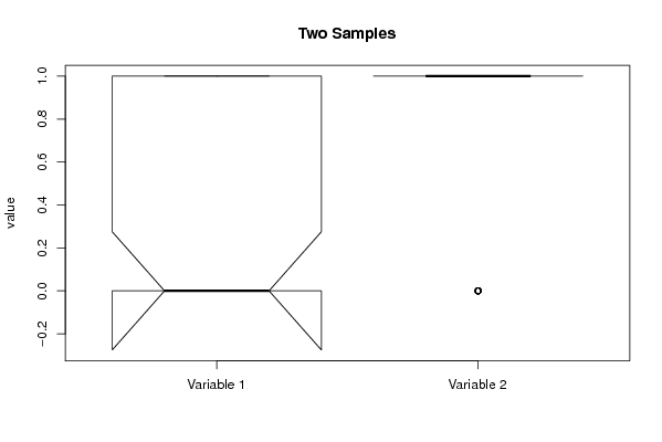
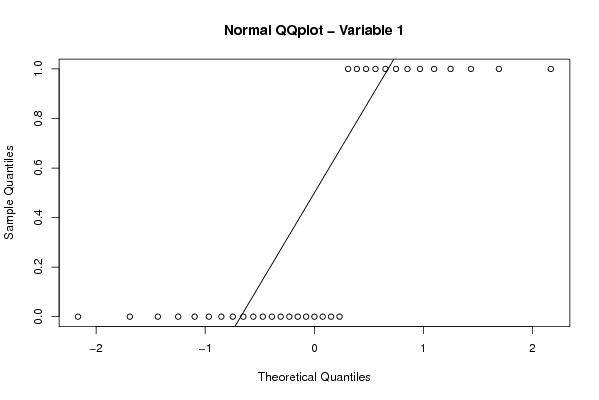
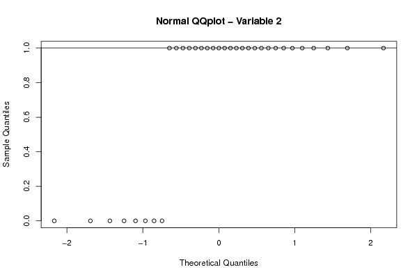
Figures (Output of Computation) | |||||||||||||||||||||||||||||||||||||||||||||||||||||||||||||||||||||||||||||||||||||||||||||||||||||||||||||||||||||||||||||||||||||||||||||||||||||||||||||||||||||||||
Input Parameters & R Code | |||||||||||||||||||||||||||||||||||||||||||||||||||||||||||||||||||||||||||||||||||||||||||||||||||||||||||||||||||||||||||||||||||||||||||||||||||||||||||||||||||||||||
| Parameters (Session): | |||||||||||||||||||||||||||||||||||||||||||||||||||||||||||||||||||||||||||||||||||||||||||||||||||||||||||||||||||||||||||||||||||||||||||||||||||||||||||||||||||||||||
| par1 = 1 ; par2 = 2 ; par3 = 0.95 ; par4 = two.sided ; par5 = paired ; par6 = 0.0 ; | |||||||||||||||||||||||||||||||||||||||||||||||||||||||||||||||||||||||||||||||||||||||||||||||||||||||||||||||||||||||||||||||||||||||||||||||||||||||||||||||||||||||||
| Parameters (R input): | |||||||||||||||||||||||||||||||||||||||||||||||||||||||||||||||||||||||||||||||||||||||||||||||||||||||||||||||||||||||||||||||||||||||||||||||||||||||||||||||||||||||||
| par1 = 1 ; par2 = 2 ; par3 = 0.95 ; par4 = two.sided ; par5 = paired ; par6 = 0.0 ; | |||||||||||||||||||||||||||||||||||||||||||||||||||||||||||||||||||||||||||||||||||||||||||||||||||||||||||||||||||||||||||||||||||||||||||||||||||||||||||||||||||||||||
| R code (references can be found in the software module): | |||||||||||||||||||||||||||||||||||||||||||||||||||||||||||||||||||||||||||||||||||||||||||||||||||||||||||||||||||||||||||||||||||||||||||||||||||||||||||||||||||||||||
par1 <- as.numeric(par1) #column number of first sample | |||||||||||||||||||||||||||||||||||||||||||||||||||||||||||||||||||||||||||||||||||||||||||||||||||||||||||||||||||||||||||||||||||||||||||||||||||||||||||||||||||||||||