Repository of Reproducible Computations

Free Statistics

of Irreproducible Research!

Author's title

Author

*The author of this computation has been verified*

R Software Module

rwasp_chi_squared_tests.wasp

Title produced by software

Chi-Squared and McNemar Tests

Date of computation

Fri, 12 Nov 2010 15:16:53 +0000

Cite this page as follows

Statistical Computations at FreeStatistics.org, Office for Research Development and Education, URL https://freestatistics.org/blog/index.php?v=date/2010/Nov/12/t12895749646dtn5nkcjmouykc.htm/, Retrieved Tue, 30 Apr 2024 18:42:28 +0000

Statistical Computations at FreeStatistics.org, Office for Research Development and Education, URL https://freestatistics.org/blog/index.php?pk=94199, Retrieved Tue, 30 Apr 2024 18:42:28 +0000

QR Codes:

Paste this QR Code to cite your computation.

Original text written by user:

IsPrivate?

No (this computation is public)

User-defined keywords

Estimated Impact

120

Family? (F = Feedback message, R = changed R code, M = changed R Module, P = changed Parameters, D = changed Data)

-     [] [WS 6 Connected vs...] [-0001-11-30 00:00:00] [8081b8996d5947580de3eb171e82db4f]
F RMPD    [Chi-Squared and McNemar Tests] [WS 6 Happiness vs...] [2010-11-12 15:16:53] [4d0f7ea43b071af5c75b527ee1ef14c2] [Current]

Feedback Forum

2010-11-21 07:53:59 [48eb36e2c01435ad7e4ea7854a9d98fe] [reply] 
De student heeft hier de correcte softwaremodule gebruikt, rekening houdend met de gegevens. We zien dat de minimale cell count van 5 ruim overschreden wordt en dus mogen we de resultaten interpreteren. 
 
De interpretatie van de P waarde werd door de student correct uitgevoerd. Nu we echter weten dat er een verband bestaat tussen beiden kunnen we kijken naar de associatie plot. Deze grafische voorstelling leert ons namelijk iets over de aard van het verband. We stellen hier vast dat het gaat om een negatief verband. Echter dienen we wel op te merken dat dit niet meteen betekent dat er ook een causaal verband bestaat tussen beiden.

Post a new message

Dataseries X:

Download CSV

Histogram

Boxplots

'HI'	'HI'
'HI'	'LO'
'LO'	'HI'
'LO'	'HI'
'HI'	'HI'
'HI'	'HI'
'HI'	'HI'
'HI'	'LO'
'HI'	'LO'
'HI'	'HI'
'HI'	'LO'
'HI'	'LO'
'LO'	'HI'
'HI'	'HI'
'HI'	'LO'
'HI'	'HI'
'HI'	'HI'
'HI'	'LO'
'HI'	'LO'
'HI'	'HI'
'HI'	'LO'
'LO'	'HI'
'HI'	'HI'
'LO'	'HI'
'HI'	'LO'
'LO'	'LO'
'HI'	'LO'
'HI'	'HI'
'HI'	'HI'
'LO'	'HI'
'HI'	'LO'
'LO'	'HI'
'HI'	'LO'
'HI'	'LO'
'HI'	'HI'
'HI'	'LO'
'LO'	'HI'
'HI'	'HI'
'HI'	'LO'
'LO'	'LO'
'HI'	'LO'
'HI'	'HI'
'HI'	'LO'
'LO'	'HI'
'LO'	'LO'
'LO'	'HI'
'HI'	'LO'
'HI'	'LO'
'HI'	'HI'
'LO'	'LO'
'HI'	'LO'
'HI'	'HI'
'LO'	'HI'
'LO'	'HI'
'LO'	'LO'
'HI'	'HI'
'HI'	'HI'
'HI'	'LO'
'LO'	'LO'
'LO'	'HI'
'LO'	'HI'
'LO'	'HI'
'LO'	'HI'
'HI'	'HI'
'HI'	'HI'
'LO'	'LO'
'LO'	'HI'
'LO'	'HI'
'HI'	'HI'
'HI'	'HI'
'HI'	'HI'
'HI'	'HI'
'HI'	'HI'
'HI'	'LO'
'LO'	'LO'
'LO'	'HI'
'HI'	'HI'
'LO'	'HI'
'HI'	'HI'
'LO'	'LO'
'HI'	'LO'
'HI'	'LO'
'HI'	'LO'
'HI'	'HI'
'HI'	'HI'
'HI'	'HI'
'HI'	'HI'
'HI'	'HI'
'LO'	'HI'
'LO'	'HI'
'HI'	'HI'
'LO'	'HI'
'HI'	'HI'
'HI'	'HI'
'LO'	'LO'
'HI'	'LO'
'LO'	'HI'
'HI'	'LO'
'HI'	'LO'
'HI'	'LO'
'HI'	'LO'
'LO'	'HI'
'HI'	'HI'
'LO'	'LO'
'HI'	'HI'
'LO'	'HI'
'HI'	'LO'
'HI'	'HI'
'LO'	'HI'
'LO'	'HI'
'HI'	'HI'
'LO'	'HI'
'LO'	'LO'
'HI'	'HI'
'HI'	'HI'
'HI'	'LO'
'HI'	'HI'
'HI'	'HI'
'HI'	'LO'
'HI'	'HI'
'LO'	'HI'
'HI'	'HI'
'HI'	'LO'
'HI'	'LO'
'HI'	'LO'
'LO'	'LO'
'HI'	'LO'
'HI'	'LO'
'HI'	'LO'
'HI'	'HI'
'LO'	'LO'
'LO'	'HI'
'HI'	'LO'
'HI'	'HI'
'HI'	'HI'
'HI'	'HI'
'LO'	'HI'
'HI'	'HI'
'LO'	'HI'
'HI'	'LO'
'LO'	'HI'
'HI'	'LO'
'HI'	'HI'
'HI'	'HI'
'HI'	'HI'
'HI'	'LO'
'HI'	'HI'
'LO'	'HI'
'LO'	'LO'
'LO'	'HI'
'HI'	'HI'
'LO'	'HI'
'HI'	'LO'
'LO'	'HI'
'LO'	'HI'
'LO'	'HI'
'LO'	'HI'
'HI'	'HI'
'HI'	'LO'
'LO'	'LO'
'LO'	'HI'
'LO'	'HI'

Summary of computational transaction
Raw Input	view raw input (R code)
Raw Output	view raw output of R engine
Computing time	2 seconds
R Server	'RServer@AstonUniversity' @ vre.aston.ac.uk

\begin{tabular}{lllllllll}
\hline
Summary of computational transaction \tabularnewline
Raw Input & view raw input (R code)  \tabularnewline
Raw Output & view raw output of R engine  \tabularnewline
Computing time & 2 seconds \tabularnewline
R Server & 'RServer@AstonUniversity' @ vre.aston.ac.uk \tabularnewline
\hline
\end{tabular}
%Source: https://freestatistics.org/blog/index.php?pk=94199&T=0

[TABLE]
[ROW][C]Summary of computational transaction[/C][/ROW]
[ROW][C]Raw Input[/C][C]view raw input (R code) [/C][/ROW]
[ROW][C]Raw Output[/C][C]view raw output of R engine [/C][/ROW]
[ROW][C]Computing time[/C][C]2 seconds[/C][/ROW]
[ROW][C]R Server[/C][C]'RServer@AstonUniversity' @ vre.aston.ac.uk[/C][/ROW]
[/TABLE]
Source: https://freestatistics.org/blog/index.php?pk=94199&T=0

Globally Unique Identifier (entire table): ba.freestatistics.org/blog/index.php?pk=94199&T=0

As an alternative you can also use a QR Code:

The GUIDs for individual cells are displayed in the table below:

Summary of computational transaction
Raw Input	view raw input (R code)
Raw Output	view raw output of R engine
Computing time	2 seconds
R Server	'RServer@AstonUniversity' @ vre.aston.ac.uk

Tabulation of Results
Hap x Depr
	HI	LO
HI	57	46
LO	43	16

\begin{tabular}{lllllllll}
\hline
Tabulation of Results \tabularnewline
Hap  x  Depr \tabularnewline
  & HI & LO \tabularnewline
HI & 57 & 46 \tabularnewline
LO & 43 & 16 \tabularnewline
\hline
\end{tabular}
%Source: https://freestatistics.org/blog/index.php?pk=94199&T=1

[TABLE]
[ROW][C]Tabulation of Results[/C][/ROW]
[ROW][C]Hap  x  Depr[/C][/ROW]
[ROW][C] [/C][C]HI[/C][C]LO[/C][/ROW]
[C]HI[/C][C]57[/C][C]46[/C][/ROW]
[C]LO[/C][C]43[/C][C]16[/C][/ROW]
[/TABLE]
Source: https://freestatistics.org/blog/index.php?pk=94199&T=1

Globally Unique Identifier (entire table): ba.freestatistics.org/blog/index.php?pk=94199&T=1

As an alternative you can also use a QR Code:

The GUIDs for individual cells are displayed in the table below:

Tabulation of Results
Hap x Depr
	HI	LO
HI	57	46
LO	43	16

Tabulation of Expected Results
Hap x Depr
	HI	LO
HI	63.58	39.42
LO	36.42	22.58

\begin{tabular}{lllllllll}
\hline
Tabulation of Expected Results \tabularnewline
Hap  x  Depr \tabularnewline
  & HI & LO \tabularnewline
HI & 63.58 & 39.42 \tabularnewline
LO & 36.42 & 22.58 \tabularnewline
\hline
\end{tabular}
%Source: https://freestatistics.org/blog/index.php?pk=94199&T=2

[TABLE]
[ROW][C]Tabulation of Expected Results[/C][/ROW]
[ROW][C]Hap  x  Depr[/C][/ROW]
[ROW][C] [/C][C]HI[/C][C]LO[/C][/ROW]
[C]HI[/C][C]63.58[/C][C]39.42[/C][/ROW]
[C]LO[/C][C]36.42[/C][C]22.58[/C][/ROW]
[/TABLE]
Source: https://freestatistics.org/blog/index.php?pk=94199&T=2

Globally Unique Identifier (entire table): ba.freestatistics.org/blog/index.php?pk=94199&T=2

As an alternative you can also use a QR Code:

The GUIDs for individual cells are displayed in the table below:

Tabulation of Expected Results
Hap x Depr
	HI	LO
HI	63.58	39.42
LO	36.42	22.58

Statistical Results
Pearson's Chi-squared test with Yates' continuity correction
Chi Square Statistic	4.17
Degrees of Freedom	1
P value	0.04

\begin{tabular}{lllllllll}
\hline
Statistical Results \tabularnewline
Pearson's Chi-squared test with Yates' continuity correction \tabularnewline
Chi Square Statistic & 4.17 \tabularnewline
Degrees of Freedom & 1 \tabularnewline
P value & 0.04 \tabularnewline
\hline
\end{tabular}
%Source: https://freestatistics.org/blog/index.php?pk=94199&T=3

[TABLE]
[ROW][C]Statistical Results[/C][/ROW]
[ROW][C]Pearson's Chi-squared test with Yates' continuity correction[/C][/ROW]
[ROW][C]Chi Square Statistic[/C][C]4.17[/C][/ROW]
[ROW][C]Degrees of Freedom[/C][C]1[/C][/ROW]
[ROW][C]P value[/C][C]0.04[/C][/ROW]
[/TABLE]
Source: https://freestatistics.org/blog/index.php?pk=94199&T=3

Globally Unique Identifier (entire table): ba.freestatistics.org/blog/index.php?pk=94199&T=3

As an alternative you can also use a QR Code:

The GUIDs for individual cells are displayed in the table below:

Statistical Results
Pearson's Chi-squared test with Yates' continuity correction
Chi Square Statistic	4.17
Degrees of Freedom	1
P value	0.04

Figure 1

PNG link

Postscript link

PDF link

Parameters (Session):

par1 = 1 ; par2 = 2 ; par3 = Pearson Chi-Squared ;

Parameters (R input):

par1 = 1 ; par2 = 2 ; par3 = Pearson Chi-Squared ;

R code (references can be found in the software module):

library(vcd)
cat1 <- as.numeric(par1) #
cat2<- as.numeric(par2) #
simulate.p.value=FALSE
if (par3 == 'Exact Pearson Chi-Squared by Simulation') simulate.p.value=TRUE
x <- t(x)
(z <- array(unlist(x),dim=c(length(x[,1]),length(x[1,]))))
(table1 <- table(z[,cat1],z[,cat2]))
(V1<-dimnames(y)[[1]][cat1])
(V2<-dimnames(y)[[1]][cat2])
bitmap(file='pic1.png')
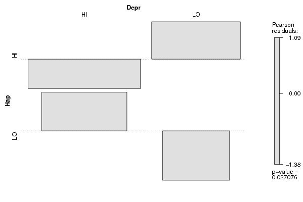
assoc(ftable(z[,cat1],z[,cat2],row.vars=1,dnn=c(V1,V2)),shade=T)
dev.off()
load(file='createtable')
a<-table.start()
a<-table.row.start(a)
a<-table.element(a,'Tabulation of Results',ncol(table1)+1,TRUE)
a<-table.row.end(a)
a<-table.row.start(a)
a<-table.element(a,paste(V1,' x ', V2),ncol(table1)+1,TRUE)
a<-table.row.end(a)
a<-table.row.start(a)
a<-table.element(a, ' ', 1,TRUE)
for(nc in 1:ncol(table1)){
a<-table.element(a, colnames(table1)[nc], 1, TRUE)
}
a<-table.row.end(a)
for(nr in 1:nrow(table1) ){
a<-table.element(a, rownames(table1)[nr], 1, TRUE)
for(nc in 1:ncol(table1) ){
a<-table.element(a, table1[nr, nc], 1, FALSE)
}
a<-table.row.end(a)
}
a<-table.end(a)
table.save(a,file='mytable.tab')
(cst<-chisq.test(table1, simulate.p.value=simulate.p.value) )
if (par3 == 'McNemar Chi-Squared') {
(cst <- mcnemar.test(table1))
}
if (par3 != 'McNemar Chi-Squared') {
a<-table.start()
a<-table.row.start(a)
a<-table.element(a,'Tabulation of Expected Results',ncol(table1)+1,TRUE)
a<-table.row.end(a)
a<-table.row.start(a)
a<-table.element(a,paste(V1,' x ', V2),ncol(table1)+1,TRUE)
a<-table.row.end(a)
a<-table.row.start(a)
a<-table.element(a, ' ', 1,TRUE)
for(nc in 1:ncol(table1)){
a<-table.element(a, colnames(table1)[nc], 1, TRUE)
}
a<-table.row.end(a)
for(nr in 1:nrow(table1) ){
a<-table.element(a, rownames(table1)[nr], 1, TRUE)
for(nc in 1:ncol(table1) ){
a<-table.element(a, round(cst$expected[nr, nc], digits=2), 1, FALSE)
}
a<-table.row.end(a)
}
a<-table.end(a)
table.save(a,file='mytable1.tab')
}
a<-table.start()
a<-table.row.start(a)
a<-table.element(a,'Statistical Results',2,TRUE)
a<-table.row.end(a)
a<-table.row.start(a)
a<-table.element(a, cst$method, 2,TRUE)
a<-table.row.end(a)
a<-table.row.start(a)
a<-table.element(a, 'Chi Square Statistic', 1, TRUE)
a<-table.element(a, round(cst$statistic, digits=2), 1,FALSE)
a<-table.row.end(a)
if(!simulate.p.value){
a<-table.row.start(a)
a<-table.element(a, 'Degrees of Freedom', 1, TRUE)
a<-table.element(a, cst$parameter, 1,FALSE)
a<-table.row.end(a)
}
a<-table.row.start(a)
a<-table.element(a, 'P value', 1, TRUE)
a<-table.element(a, round(cst$p.value, digits=2), 1,FALSE)
a<-table.row.end(a)
a<-table.end(a)
table.save(a,file='mytable2.tab')

Free Statistics

Description of Statistical Computation

Tree of Dependent Computations

Dataset

Tables (Output of Computation)

Figures (Output of Computation)

Input Parameters & R Code