Free Statistics
of Irreproducible Research!
Description of Statistical Computation | |||||||||||||||||||||
|---|---|---|---|---|---|---|---|---|---|---|---|---|---|---|---|---|---|---|---|---|---|
| Author's title | |||||||||||||||||||||
| Author | *Unverified author* | ||||||||||||||||||||
| R Software Module | rwasp_meanplot.wasp | ||||||||||||||||||||
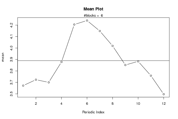
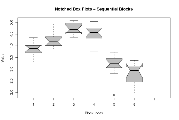
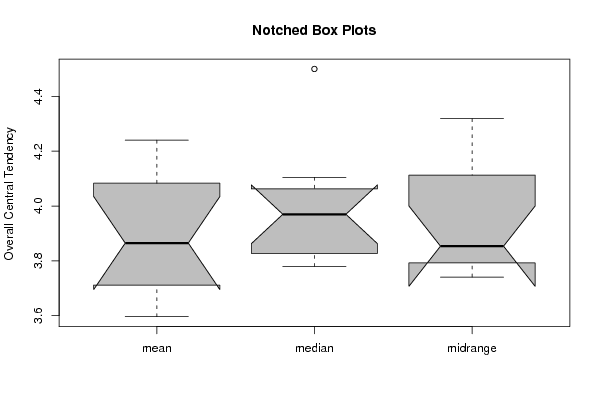
| Title produced by software | Mean Plot | ||||||||||||||||||||
| Date of computation | Mon, 15 Nov 2010 11:09:34 +0000 | ||||||||||||||||||||
| Cite this page as follows | Statistical Computations at FreeStatistics.org, Office for Research Development and Education, URL https://freestatistics.org/blog/index.php?v=date/2010/Nov/15/t1289819418ap8nv60tim1qrb1.htm/, Retrieved Sun, 28 Apr 2024 04:13:12 +0000 | ||||||||||||||||||||
| Statistical Computations at FreeStatistics.org, Office for Research Development and Education, URL https://freestatistics.org/blog/index.php?pk=94751, Retrieved Sun, 28 Apr 2024 04:13:12 +0000 | |||||||||||||||||||||
| QR Codes: | |||||||||||||||||||||
|
| |||||||||||||||||||||
| Original text written by user: | |||||||||||||||||||||
| IsPrivate? | No (this computation is public) | ||||||||||||||||||||
| User-defined keywords | KDGP1W52 | ||||||||||||||||||||
| Estimated Impact | 178 | ||||||||||||||||||||
Tree of Dependent Computations | |||||||||||||||||||||
| Family? (F = Feedback message, R = changed R code, M = changed R Module, P = changed Parameters, D = changed Data) | |||||||||||||||||||||
| - [Mean Plot] [opgave 5 oef 1 st...] [2010-01-06 15:20:10] [bca481c43219f65eca3a6066c160a58b] - PD [Mean Plot] [mean plot eige ge...] [2010-11-15 11:09:34] [9b9daabfb4dd89dd7e1d590f0423e9fb] [Current] | |||||||||||||||||||||
| Feedback Forum | |||||||||||||||||||||
Post a new message | |||||||||||||||||||||
Dataset | |||||||||||||||||||||
| Dataseries X: | |||||||||||||||||||||
3.65 3.59 3.31 3.89 4.31 4.35 4.11 3.90 3.75 3.75 3.88 3.93 3.97 3.97 4.33 4.16 4.93 3.86 4.06 4.18 4.08 4.38 4.48 4.41 4.37 4.56 4.71 4.94 5.03 5.08 5.05 4.83 4.68 4.69 4.58 4.54 4.75 4.71 4.50 4.62 4.69 5.05 4.93 4.53 4.33 4.33 3.87 3.74 3.31 3.21 2.93 3.19 3.46 3.73 3.60 3.46 3.25 3.19 2.82 1.89 1.98 2.30 2.42 2.47 2.81 3.37 3.14 3.21 3.02 2.96 2.92 3.07 | |||||||||||||||||||||
Tables (Output of Computation) | |||||||||||||||||||||
| |||||||||||||||||||||
Figures (Output of Computation) | |||||||||||||||||||||
Input Parameters & R Code | |||||||||||||||||||||
| Parameters (Session): | |||||||||||||||||||||
| par1 = 12 ; | |||||||||||||||||||||
| Parameters (R input): | |||||||||||||||||||||
| par1 = 12 ; | |||||||||||||||||||||
| R code (references can be found in the software module): | |||||||||||||||||||||
par1 <- as.numeric(par1) | |||||||||||||||||||||