Free Statistics
of Irreproducible Research!
Description of Statistical Computation | |||||||||||||||||||||
|---|---|---|---|---|---|---|---|---|---|---|---|---|---|---|---|---|---|---|---|---|---|
| Author's title | |||||||||||||||||||||
| Author | *Unverified author* | ||||||||||||||||||||
| R Software Module | rwasp_meanplot.wasp | ||||||||||||||||||||
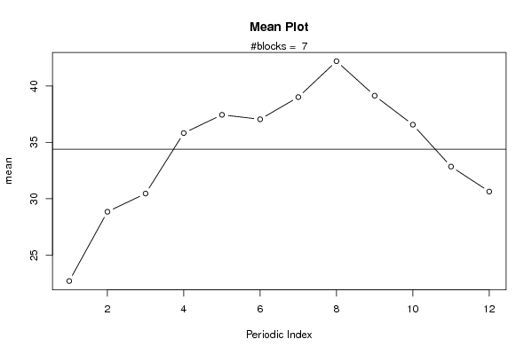
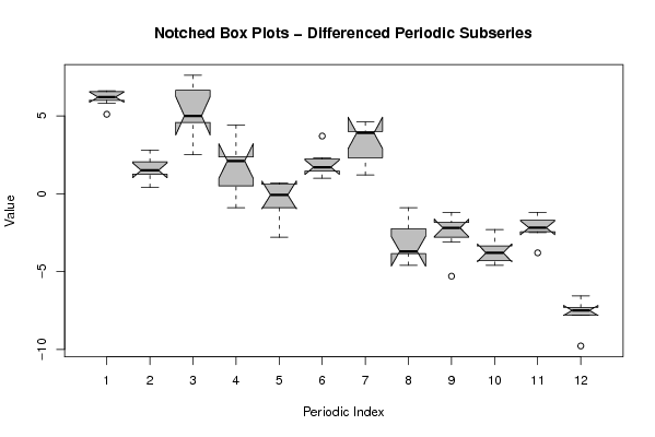
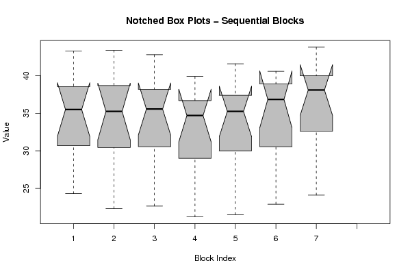
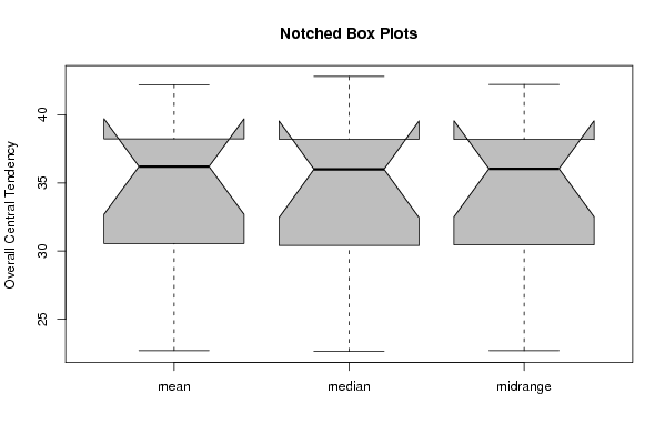
| Title produced by software | Mean Plot | ||||||||||||||||||||
| Date of computation | Mon, 15 Nov 2010 11:05:37 +0000 | ||||||||||||||||||||
| Cite this page as follows | Statistical Computations at FreeStatistics.org, Office for Research Development and Education, URL https://freestatistics.org/blog/index.php?v=date/2010/Nov/15/t1289819539bvcp64ya8rvv2wt.htm/, Retrieved Sun, 28 Apr 2024 02:58:28 +0000 | ||||||||||||||||||||
| Statistical Computations at FreeStatistics.org, Office for Research Development and Education, URL https://freestatistics.org/blog/index.php?pk=94753, Retrieved Sun, 28 Apr 2024 02:58:28 +0000 | |||||||||||||||||||||
| QR Codes: | |||||||||||||||||||||
|
| |||||||||||||||||||||
| Original text written by user: | |||||||||||||||||||||
| IsPrivate? | No (this computation is public) | ||||||||||||||||||||
| User-defined keywords | KDGP1W52 | ||||||||||||||||||||
| Estimated Impact | 167 | ||||||||||||||||||||
Tree of Dependent Computations | |||||||||||||||||||||
| Family? (F = Feedback message, R = changed R code, M = changed R Module, P = changed Parameters, D = changed Data) | |||||||||||||||||||||
| - [Univariate Data Series] [opgave 6 oef 1 ] [2010-11-15 10:03:25] [a8df0d1af66a7f69bd895162e6e9e24a] - RMPD [Mean Plot] [opgave 6 oef 2 ] [2010-11-15 11:05:37] [d5f8481d835a4a90565680e4111cba41] [Current] | |||||||||||||||||||||
| Feedback Forum | |||||||||||||||||||||
Post a new message | |||||||||||||||||||||
Dataset | |||||||||||||||||||||
| Dataseries X: | |||||||||||||||||||||
24,3 29,4 31,8 36,7 37,1 37,7 39,4 43,3 39,6 34,3 32 29,6 22,3 28,9 31,7 34,2 38,6 37,2 38,8 43,4 38,8 36,3 33 29,2 22,64 28,44 30,14 34,39 36,82 36,74 38,9 42,8 39,09 37,49 33,17 30,98 21,2 27,8 29 35,4 37,5 34,7 38,4 39,9 35,9 34,7 30,4 29 21,5 28 29,3 34,3 36,6 36,2 37,5 41,6 39,4 37,3 32,7 30,7 22,9 29,1 29,5 37,1 37,7 38,4 39,4 40,6 39,7 36,6 32,8 31,6 24,1 30,3 31,8 38,7 37,8 38,4 40,7 43,8 41,5 39,3 35,9 33,4 | |||||||||||||||||||||
Tables (Output of Computation) | |||||||||||||||||||||
| |||||||||||||||||||||
Figures (Output of Computation) | |||||||||||||||||||||
Input Parameters & R Code | |||||||||||||||||||||
| Parameters (Session): | |||||||||||||||||||||
| par1 = 12 ; | |||||||||||||||||||||
| Parameters (R input): | |||||||||||||||||||||
| par1 = 12 ; | |||||||||||||||||||||
| R code (references can be found in the software module): | |||||||||||||||||||||
par1 <- as.numeric(par1) | |||||||||||||||||||||