Repository of Reproducible Computations

Free Statistics

of Irreproducible Research!

Author's title

Author

*Unverified author*

R Software Module

rwasp_autocorrelation.wasp

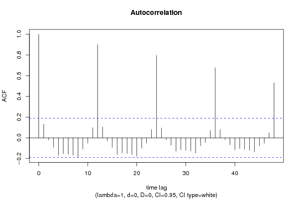
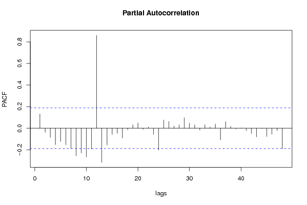
Title produced by software

(Partial) Autocorrelation Function

Date of computation

Mon, 15 Nov 2010 14:56:33 +0000

Cite this page as follows

Statistical Computations at FreeStatistics.org, Office for Research Development and Education, URL https://freestatistics.org/blog/index.php?v=date/2010/Nov/15/t1289832975wqg0wgbxjv5plkj.htm/, Retrieved Sun, 28 Apr 2024 17:12:04 +0000

Statistical Computations at FreeStatistics.org, Office for Research Development and Education, URL https://freestatistics.org/blog/index.php?pk=94862, Retrieved Sun, 28 Apr 2024 17:12:04 +0000

QR Codes:

Paste this QR Code to cite your computation.

Original text written by user:

IsPrivate?

No (this computation is public)

User-defined keywords

KDGP2W12

Estimated Impact

102

Family? (F = Feedback message, R = changed R code, M = changed R Module, P = changed Parameters, D = changed Data)

-       [(Partial) Autocorrelation Function] [opdracht 6 bis ei...] [2010-11-15 14:56:33] [208cd78e8ef15d69f7248238ad0efe72] [Current]

Feedback Forum

Post a new message

Dataseries X:

Download CSV

Histogram

Boxplots

Summary of computational transaction
Raw Input	view raw input (R code)
Raw Output	view raw output of R engine
Computing time	1 seconds
R Server	'George Udny Yule' @ 72.249.76.132

\begin{tabular}{lllllllll}
\hline
Summary of computational transaction \tabularnewline
Raw Input & view raw input (R code)  \tabularnewline
Raw Output & view raw output of R engine  \tabularnewline
Computing time & 1 seconds \tabularnewline
R Server & 'George Udny Yule' @ 72.249.76.132 \tabularnewline
\hline
\end{tabular}
%Source: https://freestatistics.org/blog/index.php?pk=94862&T=0

[TABLE]
[ROW][C]Summary of computational transaction[/C][/ROW]
[ROW][C]Raw Input[/C][C]view raw input (R code) [/C][/ROW]
[ROW][C]Raw Output[/C][C]view raw output of R engine [/C][/ROW]
[ROW][C]Computing time[/C][C]1 seconds[/C][/ROW]
[ROW][C]R Server[/C][C]'George Udny Yule' @ 72.249.76.132[/C][/ROW]
[/TABLE]
Source: https://freestatistics.org/blog/index.php?pk=94862&T=0

Globally Unique Identifier (entire table): ba.freestatistics.org/blog/index.php?pk=94862&T=0

As an alternative you can also use a QR Code:

The GUIDs for individual cells are displayed in the table below:

Summary of computational transaction
Raw Input	view raw input (R code)
Raw Output	view raw output of R engine
Computing time	1 seconds
R Server	'George Udny Yule' @ 72.249.76.132

Autocorrelation Function
Time lag k	ACF(k)	T-STAT	P-value
1	0.132389	1.3758	0.085861
2	-0.020452	-0.2125	0.416043
3	-0.091719	-0.9532	0.171316
4	-0.171307	-1.7803	0.038921
5	-0.153163	-1.5917	0.057186
6	-0.159647	-1.6591	0.049998
7	-0.168103	-1.747	0.041742
8	-0.190346	-1.9781	0.02523
9	-0.109638	-1.1394	0.12853
10	-0.052104	-0.5415	0.294644
11	0.097712	1.0155	0.156079
12	0.900764	9.361	0
13	0.104558	1.0866	0.139816
14	-0.029995	-0.3117	0.377926
15	-0.09292	-0.9657	0.168187
16	-0.160876	-1.6719	0.048722
17	-0.146921	-1.5268	0.064861
18	-0.152906	-1.589	0.057487
19	-0.161322	-1.6765	0.048266
20	-0.176755	-1.8369	0.034488
21	-0.099689	-1.036	0.151258
22	-0.053244	-0.5533	0.290591
23	0.081135	0.8432	0.200496
24	0.796669	8.2792	0
25	0.095993	0.9976	0.160354
26	-0.017336	-0.1802	0.428682
27	-0.072269	-0.751	0.227131
28	-0.130388	-1.355	0.089118
29	-0.114962	-1.1947	0.117406
30	-0.12095	-1.2569	0.105742
31	-0.128542	-1.3359	0.092203
32	-0.148046	-1.5385	0.063421
33	-0.077453	-0.8049	0.211318
34	-0.045188	-0.4696	0.319791
35	0.070728	0.735	0.231958
36	0.676939	7.035	0
37	0.080154	0.833	0.203346
38	-0.017758	-0.1845	0.426966
39	-0.068216	-0.7089	0.239951
40	-0.116445	-1.2101	0.114435
41	-0.103603	-1.0767	0.142012
42	-0.111027	-1.1538	0.12556
43	-0.122005	-1.2679	0.103777
44	-0.137093	-1.4247	0.078561
45	-0.079369	-0.8248	0.205644
46	-0.053688	-0.5579	0.28902
47	0.049875	0.5183	0.302648
48	0.531833	5.527	0

\begin{tabular}{lllllllll}
\hline
Autocorrelation Function \tabularnewline
Time lag k & ACF(k) & T-STAT & P-value \tabularnewline
1 & 0.132389 & 1.3758 & 0.085861 \tabularnewline
2 & -0.020452 & -0.2125 & 0.416043 \tabularnewline
3 & -0.091719 & -0.9532 & 0.171316 \tabularnewline
4 & -0.171307 & -1.7803 & 0.038921 \tabularnewline
5 & -0.153163 & -1.5917 & 0.057186 \tabularnewline
6 & -0.159647 & -1.6591 & 0.049998 \tabularnewline
7 & -0.168103 & -1.747 & 0.041742 \tabularnewline
8 & -0.190346 & -1.9781 & 0.02523 \tabularnewline
9 & -0.109638 & -1.1394 & 0.12853 \tabularnewline
10 & -0.052104 & -0.5415 & 0.294644 \tabularnewline
11 & 0.097712 & 1.0155 & 0.156079 \tabularnewline
12 & 0.900764 & 9.361 & 0 \tabularnewline
13 & 0.104558 & 1.0866 & 0.139816 \tabularnewline
14 & -0.029995 & -0.3117 & 0.377926 \tabularnewline
15 & -0.09292 & -0.9657 & 0.168187 \tabularnewline
16 & -0.160876 & -1.6719 & 0.048722 \tabularnewline
17 & -0.146921 & -1.5268 & 0.064861 \tabularnewline
18 & -0.152906 & -1.589 & 0.057487 \tabularnewline
19 & -0.161322 & -1.6765 & 0.048266 \tabularnewline
20 & -0.176755 & -1.8369 & 0.034488 \tabularnewline
21 & -0.099689 & -1.036 & 0.151258 \tabularnewline
22 & -0.053244 & -0.5533 & 0.290591 \tabularnewline
23 & 0.081135 & 0.8432 & 0.200496 \tabularnewline
24 & 0.796669 & 8.2792 & 0 \tabularnewline
25 & 0.095993 & 0.9976 & 0.160354 \tabularnewline
26 & -0.017336 & -0.1802 & 0.428682 \tabularnewline
27 & -0.072269 & -0.751 & 0.227131 \tabularnewline
28 & -0.130388 & -1.355 & 0.089118 \tabularnewline
29 & -0.114962 & -1.1947 & 0.117406 \tabularnewline
30 & -0.12095 & -1.2569 & 0.105742 \tabularnewline
31 & -0.128542 & -1.3359 & 0.092203 \tabularnewline
32 & -0.148046 & -1.5385 & 0.063421 \tabularnewline
33 & -0.077453 & -0.8049 & 0.211318 \tabularnewline
34 & -0.045188 & -0.4696 & 0.319791 \tabularnewline
35 & 0.070728 & 0.735 & 0.231958 \tabularnewline
36 & 0.676939 & 7.035 & 0 \tabularnewline
37 & 0.080154 & 0.833 & 0.203346 \tabularnewline
38 & -0.017758 & -0.1845 & 0.426966 \tabularnewline
39 & -0.068216 & -0.7089 & 0.239951 \tabularnewline
40 & -0.116445 & -1.2101 & 0.114435 \tabularnewline
41 & -0.103603 & -1.0767 & 0.142012 \tabularnewline
42 & -0.111027 & -1.1538 & 0.12556 \tabularnewline
43 & -0.122005 & -1.2679 & 0.103777 \tabularnewline
44 & -0.137093 & -1.4247 & 0.078561 \tabularnewline
45 & -0.079369 & -0.8248 & 0.205644 \tabularnewline
46 & -0.053688 & -0.5579 & 0.28902 \tabularnewline
47 & 0.049875 & 0.5183 & 0.302648 \tabularnewline
48 & 0.531833 & 5.527 & 0 \tabularnewline
\hline
\end{tabular}
%Source: https://freestatistics.org/blog/index.php?pk=94862&T=1

[TABLE]
[ROW][C]Autocorrelation Function[/C][/ROW]
[ROW][C]Time lag k[/C][C]ACF(k)[/C][C]T-STAT[/C][C]P-value[/C][/ROW]
[ROW][C]1[/C][C]0.132389[/C][C]1.3758[/C][C]0.085861[/C][/ROW]
[ROW][C]2[/C][C]-0.020452[/C][C]-0.2125[/C][C]0.416043[/C][/ROW]
[ROW][C]3[/C][C]-0.091719[/C][C]-0.9532[/C][C]0.171316[/C][/ROW]
[ROW][C]4[/C][C]-0.171307[/C][C]-1.7803[/C][C]0.038921[/C][/ROW]
[ROW][C]5[/C][C]-0.153163[/C][C]-1.5917[/C][C]0.057186[/C][/ROW]
[ROW][C]6[/C][C]-0.159647[/C][C]-1.6591[/C][C]0.049998[/C][/ROW]
[ROW][C]7[/C][C]-0.168103[/C][C]-1.747[/C][C]0.041742[/C][/ROW]
[ROW][C]8[/C][C]-0.190346[/C][C]-1.9781[/C][C]0.02523[/C][/ROW]
[ROW][C]9[/C][C]-0.109638[/C][C]-1.1394[/C][C]0.12853[/C][/ROW]
[ROW][C]10[/C][C]-0.052104[/C][C]-0.5415[/C][C]0.294644[/C][/ROW]
[ROW][C]11[/C][C]0.097712[/C][C]1.0155[/C][C]0.156079[/C][/ROW]
[ROW][C]12[/C][C]0.900764[/C][C]9.361[/C][C]0[/C][/ROW]
[ROW][C]13[/C][C]0.104558[/C][C]1.0866[/C][C]0.139816[/C][/ROW]
[ROW][C]14[/C][C]-0.029995[/C][C]-0.3117[/C][C]0.377926[/C][/ROW]
[ROW][C]15[/C][C]-0.09292[/C][C]-0.9657[/C][C]0.168187[/C][/ROW]
[ROW][C]16[/C][C]-0.160876[/C][C]-1.6719[/C][C]0.048722[/C][/ROW]
[ROW][C]17[/C][C]-0.146921[/C][C]-1.5268[/C][C]0.064861[/C][/ROW]
[ROW][C]18[/C][C]-0.152906[/C][C]-1.589[/C][C]0.057487[/C][/ROW]
[ROW][C]19[/C][C]-0.161322[/C][C]-1.6765[/C][C]0.048266[/C][/ROW]
[ROW][C]20[/C][C]-0.176755[/C][C]-1.8369[/C][C]0.034488[/C][/ROW]
[ROW][C]21[/C][C]-0.099689[/C][C]-1.036[/C][C]0.151258[/C][/ROW]
[ROW][C]22[/C][C]-0.053244[/C][C]-0.5533[/C][C]0.290591[/C][/ROW]
[ROW][C]23[/C][C]0.081135[/C][C]0.8432[/C][C]0.200496[/C][/ROW]
[ROW][C]24[/C][C]0.796669[/C][C]8.2792[/C][C]0[/C][/ROW]
[ROW][C]25[/C][C]0.095993[/C][C]0.9976[/C][C]0.160354[/C][/ROW]
[ROW][C]26[/C][C]-0.017336[/C][C]-0.1802[/C][C]0.428682[/C][/ROW]
[ROW][C]27[/C][C]-0.072269[/C][C]-0.751[/C][C]0.227131[/C][/ROW]
[ROW][C]28[/C][C]-0.130388[/C][C]-1.355[/C][C]0.089118[/C][/ROW]
[ROW][C]29[/C][C]-0.114962[/C][C]-1.1947[/C][C]0.117406[/C][/ROW]
[ROW][C]30[/C][C]-0.12095[/C][C]-1.2569[/C][C]0.105742[/C][/ROW]
[ROW][C]31[/C][C]-0.128542[/C][C]-1.3359[/C][C]0.092203[/C][/ROW]
[ROW][C]32[/C][C]-0.148046[/C][C]-1.5385[/C][C]0.063421[/C][/ROW]
[ROW][C]33[/C][C]-0.077453[/C][C]-0.8049[/C][C]0.211318[/C][/ROW]
[ROW][C]34[/C][C]-0.045188[/C][C]-0.4696[/C][C]0.319791[/C][/ROW]
[ROW][C]35[/C][C]0.070728[/C][C]0.735[/C][C]0.231958[/C][/ROW]
[ROW][C]36[/C][C]0.676939[/C][C]7.035[/C][C]0[/C][/ROW]
[ROW][C]37[/C][C]0.080154[/C][C]0.833[/C][C]0.203346[/C][/ROW]
[ROW][C]38[/C][C]-0.017758[/C][C]-0.1845[/C][C]0.426966[/C][/ROW]
[ROW][C]39[/C][C]-0.068216[/C][C]-0.7089[/C][C]0.239951[/C][/ROW]
[ROW][C]40[/C][C]-0.116445[/C][C]-1.2101[/C][C]0.114435[/C][/ROW]
[ROW][C]41[/C][C]-0.103603[/C][C]-1.0767[/C][C]0.142012[/C][/ROW]
[ROW][C]42[/C][C]-0.111027[/C][C]-1.1538[/C][C]0.12556[/C][/ROW]
[ROW][C]43[/C][C]-0.122005[/C][C]-1.2679[/C][C]0.103777[/C][/ROW]
[ROW][C]44[/C][C]-0.137093[/C][C]-1.4247[/C][C]0.078561[/C][/ROW]
[ROW][C]45[/C][C]-0.079369[/C][C]-0.8248[/C][C]0.205644[/C][/ROW]
[ROW][C]46[/C][C]-0.053688[/C][C]-0.5579[/C][C]0.28902[/C][/ROW]
[ROW][C]47[/C][C]0.049875[/C][C]0.5183[/C][C]0.302648[/C][/ROW]
[ROW][C]48[/C][C]0.531833[/C][C]5.527[/C][C]0[/C][/ROW]
[/TABLE]
Source: https://freestatistics.org/blog/index.php?pk=94862&T=1

Globally Unique Identifier (entire table): ba.freestatistics.org/blog/index.php?pk=94862&T=1

As an alternative you can also use a QR Code:

The GUIDs for individual cells are displayed in the table below:

Autocorrelation Function
Time lag k	ACF(k)	T-STAT	P-value
1	0.132389	1.3758	0.085861
2	-0.020452	-0.2125	0.416043
3	-0.091719	-0.9532	0.171316
4	-0.171307	-1.7803	0.038921
5	-0.153163	-1.5917	0.057186
6	-0.159647	-1.6591	0.049998
7	-0.168103	-1.747	0.041742
8	-0.190346	-1.9781	0.02523
9	-0.109638	-1.1394	0.12853
10	-0.052104	-0.5415	0.294644
11	0.097712	1.0155	0.156079
12	0.900764	9.361	0
13	0.104558	1.0866	0.139816
14	-0.029995	-0.3117	0.377926
15	-0.09292	-0.9657	0.168187
16	-0.160876	-1.6719	0.048722
17	-0.146921	-1.5268	0.064861
18	-0.152906	-1.589	0.057487
19	-0.161322	-1.6765	0.048266
20	-0.176755	-1.8369	0.034488
21	-0.099689	-1.036	0.151258
22	-0.053244	-0.5533	0.290591
23	0.081135	0.8432	0.200496
24	0.796669	8.2792	0
25	0.095993	0.9976	0.160354
26	-0.017336	-0.1802	0.428682
27	-0.072269	-0.751	0.227131
28	-0.130388	-1.355	0.089118
29	-0.114962	-1.1947	0.117406
30	-0.12095	-1.2569	0.105742
31	-0.128542	-1.3359	0.092203
32	-0.148046	-1.5385	0.063421
33	-0.077453	-0.8049	0.211318
34	-0.045188	-0.4696	0.319791
35	0.070728	0.735	0.231958
36	0.676939	7.035	0
37	0.080154	0.833	0.203346
38	-0.017758	-0.1845	0.426966
39	-0.068216	-0.7089	0.239951
40	-0.116445	-1.2101	0.114435
41	-0.103603	-1.0767	0.142012
42	-0.111027	-1.1538	0.12556
43	-0.122005	-1.2679	0.103777
44	-0.137093	-1.4247	0.078561
45	-0.079369	-0.8248	0.205644
46	-0.053688	-0.5579	0.28902
47	0.049875	0.5183	0.302648
48	0.531833	5.527	0

Partial Autocorrelation Function
Time lag k	PACF(k)	T-STAT	P-value
1	0.132389	1.3758	0.085861
2	-0.038656	-0.4017	0.34434
3	-0.085411	-0.8876	0.188358
4	-0.152222	-1.5819	0.058294
5	-0.122382	-1.2718	0.103082
6	-0.153171	-1.5918	0.057176
7	-0.188568	-1.9597	0.026306
8	-0.256059	-2.661	0.004489
9	-0.229231	-2.3822	0.009478
10	-0.266712	-2.7717	0.003284
11	-0.192085	-1.9962	0.024214
12	0.860808	8.9458	0
13	-0.315676	-3.2806	0.000698
14	-0.155262	-1.6135	0.054774
15	-0.058352	-0.6064	0.272758
16	-0.047606	-0.4947	0.310896
17	-0.090686	-0.9424	0.174037
18	-0.014141	-0.147	0.441719
19	0.031529	0.3277	0.3719
20	0.048102	0.4999	0.309086
21	-0.010693	-0.1111	0.455861
22	0.010866	0.1129	0.45515
23	-0.057927	-0.602	0.274219
24	-0.203294	-2.1127	0.018466
25	0.076637	0.7964	0.213763
26	0.062454	0.649	0.258845
27	0.019607	0.2038	0.419461
28	0.032051	0.3331	0.369859
29	0.097471	1.0129	0.156675
30	0.048287	0.5018	0.308411
31	0.030724	0.3193	0.375062
32	-0.016433	-0.1708	0.43236
33	0.033344	0.3465	0.364814
34	0.011591	0.1205	0.452171
35	0.039517	0.4107	0.341064
36	-0.107778	-1.1201	0.132586
37	0.061085	0.6348	0.263445
38	0.017153	0.1783	0.429426
39	-0.0067	-0.0696	0.472309
40	0.002215	0.023	0.490837
41	-0.022998	-0.239	0.405778
42	-0.049587	-0.5153	0.30369
43	-0.080362	-0.8351	0.20274
44	-0.003133	-0.0326	0.487043
45	-0.07706	-0.8008	0.212493
46	-0.056169	-0.5837	0.280311
47	-0.022211	-0.2308	0.408943
48	-0.189927	-1.9738	0.02548

\begin{tabular}{lllllllll}
\hline
Partial Autocorrelation Function \tabularnewline
Time lag k & PACF(k) & T-STAT & P-value \tabularnewline
1 & 0.132389 & 1.3758 & 0.085861 \tabularnewline
2 & -0.038656 & -0.4017 & 0.34434 \tabularnewline
3 & -0.085411 & -0.8876 & 0.188358 \tabularnewline
4 & -0.152222 & -1.5819 & 0.058294 \tabularnewline
5 & -0.122382 & -1.2718 & 0.103082 \tabularnewline
6 & -0.153171 & -1.5918 & 0.057176 \tabularnewline
7 & -0.188568 & -1.9597 & 0.026306 \tabularnewline
8 & -0.256059 & -2.661 & 0.004489 \tabularnewline
9 & -0.229231 & -2.3822 & 0.009478 \tabularnewline
10 & -0.266712 & -2.7717 & 0.003284 \tabularnewline
11 & -0.192085 & -1.9962 & 0.024214 \tabularnewline
12 & 0.860808 & 8.9458 & 0 \tabularnewline
13 & -0.315676 & -3.2806 & 0.000698 \tabularnewline
14 & -0.155262 & -1.6135 & 0.054774 \tabularnewline
15 & -0.058352 & -0.6064 & 0.272758 \tabularnewline
16 & -0.047606 & -0.4947 & 0.310896 \tabularnewline
17 & -0.090686 & -0.9424 & 0.174037 \tabularnewline
18 & -0.014141 & -0.147 & 0.441719 \tabularnewline
19 & 0.031529 & 0.3277 & 0.3719 \tabularnewline
20 & 0.048102 & 0.4999 & 0.309086 \tabularnewline
21 & -0.010693 & -0.1111 & 0.455861 \tabularnewline
22 & 0.010866 & 0.1129 & 0.45515 \tabularnewline
23 & -0.057927 & -0.602 & 0.274219 \tabularnewline
24 & -0.203294 & -2.1127 & 0.018466 \tabularnewline
25 & 0.076637 & 0.7964 & 0.213763 \tabularnewline
26 & 0.062454 & 0.649 & 0.258845 \tabularnewline
27 & 0.019607 & 0.2038 & 0.419461 \tabularnewline
28 & 0.032051 & 0.3331 & 0.369859 \tabularnewline
29 & 0.097471 & 1.0129 & 0.156675 \tabularnewline
30 & 0.048287 & 0.5018 & 0.308411 \tabularnewline
31 & 0.030724 & 0.3193 & 0.375062 \tabularnewline
32 & -0.016433 & -0.1708 & 0.43236 \tabularnewline
33 & 0.033344 & 0.3465 & 0.364814 \tabularnewline
34 & 0.011591 & 0.1205 & 0.452171 \tabularnewline
35 & 0.039517 & 0.4107 & 0.341064 \tabularnewline
36 & -0.107778 & -1.1201 & 0.132586 \tabularnewline
37 & 0.061085 & 0.6348 & 0.263445 \tabularnewline
38 & 0.017153 & 0.1783 & 0.429426 \tabularnewline
39 & -0.0067 & -0.0696 & 0.472309 \tabularnewline
40 & 0.002215 & 0.023 & 0.490837 \tabularnewline
41 & -0.022998 & -0.239 & 0.405778 \tabularnewline
42 & -0.049587 & -0.5153 & 0.30369 \tabularnewline
43 & -0.080362 & -0.8351 & 0.20274 \tabularnewline
44 & -0.003133 & -0.0326 & 0.487043 \tabularnewline
45 & -0.07706 & -0.8008 & 0.212493 \tabularnewline
46 & -0.056169 & -0.5837 & 0.280311 \tabularnewline
47 & -0.022211 & -0.2308 & 0.408943 \tabularnewline
48 & -0.189927 & -1.9738 & 0.02548 \tabularnewline
\hline
\end{tabular}
%Source: https://freestatistics.org/blog/index.php?pk=94862&T=2

[TABLE]
[ROW][C]Partial Autocorrelation Function[/C][/ROW]
[ROW][C]Time lag k[/C][C]PACF(k)[/C][C]T-STAT[/C][C]P-value[/C][/ROW]
[ROW][C]1[/C][C]0.132389[/C][C]1.3758[/C][C]0.085861[/C][/ROW]
[ROW][C]2[/C][C]-0.038656[/C][C]-0.4017[/C][C]0.34434[/C][/ROW]
[ROW][C]3[/C][C]-0.085411[/C][C]-0.8876[/C][C]0.188358[/C][/ROW]
[ROW][C]4[/C][C]-0.152222[/C][C]-1.5819[/C][C]0.058294[/C][/ROW]
[ROW][C]5[/C][C]-0.122382[/C][C]-1.2718[/C][C]0.103082[/C][/ROW]
[ROW][C]6[/C][C]-0.153171[/C][C]-1.5918[/C][C]0.057176[/C][/ROW]
[ROW][C]7[/C][C]-0.188568[/C][C]-1.9597[/C][C]0.026306[/C][/ROW]
[ROW][C]8[/C][C]-0.256059[/C][C]-2.661[/C][C]0.004489[/C][/ROW]
[ROW][C]9[/C][C]-0.229231[/C][C]-2.3822[/C][C]0.009478[/C][/ROW]
[ROW][C]10[/C][C]-0.266712[/C][C]-2.7717[/C][C]0.003284[/C][/ROW]
[ROW][C]11[/C][C]-0.192085[/C][C]-1.9962[/C][C]0.024214[/C][/ROW]
[ROW][C]12[/C][C]0.860808[/C][C]8.9458[/C][C]0[/C][/ROW]
[ROW][C]13[/C][C]-0.315676[/C][C]-3.2806[/C][C]0.000698[/C][/ROW]
[ROW][C]14[/C][C]-0.155262[/C][C]-1.6135[/C][C]0.054774[/C][/ROW]
[ROW][C]15[/C][C]-0.058352[/C][C]-0.6064[/C][C]0.272758[/C][/ROW]
[ROW][C]16[/C][C]-0.047606[/C][C]-0.4947[/C][C]0.310896[/C][/ROW]
[ROW][C]17[/C][C]-0.090686[/C][C]-0.9424[/C][C]0.174037[/C][/ROW]
[ROW][C]18[/C][C]-0.014141[/C][C]-0.147[/C][C]0.441719[/C][/ROW]
[ROW][C]19[/C][C]0.031529[/C][C]0.3277[/C][C]0.3719[/C][/ROW]
[ROW][C]20[/C][C]0.048102[/C][C]0.4999[/C][C]0.309086[/C][/ROW]
[ROW][C]21[/C][C]-0.010693[/C][C]-0.1111[/C][C]0.455861[/C][/ROW]
[ROW][C]22[/C][C]0.010866[/C][C]0.1129[/C][C]0.45515[/C][/ROW]
[ROW][C]23[/C][C]-0.057927[/C][C]-0.602[/C][C]0.274219[/C][/ROW]
[ROW][C]24[/C][C]-0.203294[/C][C]-2.1127[/C][C]0.018466[/C][/ROW]
[ROW][C]25[/C][C]0.076637[/C][C]0.7964[/C][C]0.213763[/C][/ROW]
[ROW][C]26[/C][C]0.062454[/C][C]0.649[/C][C]0.258845[/C][/ROW]
[ROW][C]27[/C][C]0.019607[/C][C]0.2038[/C][C]0.419461[/C][/ROW]
[ROW][C]28[/C][C]0.032051[/C][C]0.3331[/C][C]0.369859[/C][/ROW]
[ROW][C]29[/C][C]0.097471[/C][C]1.0129[/C][C]0.156675[/C][/ROW]
[ROW][C]30[/C][C]0.048287[/C][C]0.5018[/C][C]0.308411[/C][/ROW]
[ROW][C]31[/C][C]0.030724[/C][C]0.3193[/C][C]0.375062[/C][/ROW]
[ROW][C]32[/C][C]-0.016433[/C][C]-0.1708[/C][C]0.43236[/C][/ROW]
[ROW][C]33[/C][C]0.033344[/C][C]0.3465[/C][C]0.364814[/C][/ROW]
[ROW][C]34[/C][C]0.011591[/C][C]0.1205[/C][C]0.452171[/C][/ROW]
[ROW][C]35[/C][C]0.039517[/C][C]0.4107[/C][C]0.341064[/C][/ROW]
[ROW][C]36[/C][C]-0.107778[/C][C]-1.1201[/C][C]0.132586[/C][/ROW]
[ROW][C]37[/C][C]0.061085[/C][C]0.6348[/C][C]0.263445[/C][/ROW]
[ROW][C]38[/C][C]0.017153[/C][C]0.1783[/C][C]0.429426[/C][/ROW]
[ROW][C]39[/C][C]-0.0067[/C][C]-0.0696[/C][C]0.472309[/C][/ROW]
[ROW][C]40[/C][C]0.002215[/C][C]0.023[/C][C]0.490837[/C][/ROW]
[ROW][C]41[/C][C]-0.022998[/C][C]-0.239[/C][C]0.405778[/C][/ROW]
[ROW][C]42[/C][C]-0.049587[/C][C]-0.5153[/C][C]0.30369[/C][/ROW]
[ROW][C]43[/C][C]-0.080362[/C][C]-0.8351[/C][C]0.20274[/C][/ROW]
[ROW][C]44[/C][C]-0.003133[/C][C]-0.0326[/C][C]0.487043[/C][/ROW]
[ROW][C]45[/C][C]-0.07706[/C][C]-0.8008[/C][C]0.212493[/C][/ROW]
[ROW][C]46[/C][C]-0.056169[/C][C]-0.5837[/C][C]0.280311[/C][/ROW]
[ROW][C]47[/C][C]-0.022211[/C][C]-0.2308[/C][C]0.408943[/C][/ROW]
[ROW][C]48[/C][C]-0.189927[/C][C]-1.9738[/C][C]0.02548[/C][/ROW]
[/TABLE]
Source: https://freestatistics.org/blog/index.php?pk=94862&T=2

Globally Unique Identifier (entire table): ba.freestatistics.org/blog/index.php?pk=94862&T=2

As an alternative you can also use a QR Code:

The GUIDs for individual cells are displayed in the table below:

Partial Autocorrelation Function
Time lag k	PACF(k)	T-STAT	P-value
1	0.132389	1.3758	0.085861
2	-0.038656	-0.4017	0.34434
3	-0.085411	-0.8876	0.188358
4	-0.152222	-1.5819	0.058294
5	-0.122382	-1.2718	0.103082
6	-0.153171	-1.5918	0.057176
7	-0.188568	-1.9597	0.026306
8	-0.256059	-2.661	0.004489
9	-0.229231	-2.3822	0.009478
10	-0.266712	-2.7717	0.003284
11	-0.192085	-1.9962	0.024214
12	0.860808	8.9458	0
13	-0.315676	-3.2806	0.000698
14	-0.155262	-1.6135	0.054774
15	-0.058352	-0.6064	0.272758
16	-0.047606	-0.4947	0.310896
17	-0.090686	-0.9424	0.174037
18	-0.014141	-0.147	0.441719
19	0.031529	0.3277	0.3719
20	0.048102	0.4999	0.309086
21	-0.010693	-0.1111	0.455861
22	0.010866	0.1129	0.45515
23	-0.057927	-0.602	0.274219
24	-0.203294	-2.1127	0.018466
25	0.076637	0.7964	0.213763
26	0.062454	0.649	0.258845
27	0.019607	0.2038	0.419461
28	0.032051	0.3331	0.369859
29	0.097471	1.0129	0.156675
30	0.048287	0.5018	0.308411
31	0.030724	0.3193	0.375062
32	-0.016433	-0.1708	0.43236
33	0.033344	0.3465	0.364814
34	0.011591	0.1205	0.452171
35	0.039517	0.4107	0.341064
36	-0.107778	-1.1201	0.132586
37	0.061085	0.6348	0.263445
38	0.017153	0.1783	0.429426
39	-0.0067	-0.0696	0.472309
40	0.002215	0.023	0.490837
41	-0.022998	-0.239	0.405778
42	-0.049587	-0.5153	0.30369
43	-0.080362	-0.8351	0.20274
44	-0.003133	-0.0326	0.487043
45	-0.07706	-0.8008	0.212493
46	-0.056169	-0.5837	0.280311
47	-0.022211	-0.2308	0.408943
48	-0.189927	-1.9738	0.02548

Figure 1

PNG link

Postscript link

PDF link

Figure 2

PNG link

Postscript link

PDF link

Parameters (Session):

par1 = 48 ; par2 = 1 ; par3 = 0 ; par4 = 0 ; par5 = 12 ; par6 = White Noise ; par7 = 0.95 ;

Parameters (R input):

par1 = 48 ; par2 = 1 ; par3 = 0 ; par4 = 0 ; par5 = 12 ; par6 = White Noise ; par7 = 0.95 ;

R code (references can be found in the software module):

if (par1 == 'Default') {
par1 = 10*log10(length(x))
} else {
par1 <- as.numeric(par1)
}
par2 <- as.numeric(par2)
par3 <- as.numeric(par3)
par4 <- as.numeric(par4)
par5 <- as.numeric(par5)
if (par6 == 'White Noise') par6 <- 'white' else par6 <- 'ma'
par7 <- as.numeric(par7)
if (par2 == 0) {
x <- log(x)
} else {
x <- (x ^ par2 - 1) / par2
}
if (par3 > 0) x <- diff(x,lag=1,difference=par3)
if (par4 > 0) x <- diff(x,lag=par5,difference=par4)
bitmap(file='pic1.png')
racf <- acf(x, par1, main='Autocorrelation', xlab='time lag', ylab='ACF', ci.type=par6, ci=par7, sub=paste('(lambda=',par2,', d=',par3,', D=',par4,', CI=', par7, ', CI type=',par6,')',sep=''))
dev.off()
bitmap(file='pic2.png')
rpacf <- pacf(x,par1,main='Partial Autocorrelation',xlab='lags',ylab='PACF')
dev.off()
(myacf <- c(racf$acf))
(mypacf <- c(rpacf$acf))
lengthx <- length(x)
sqrtn <- sqrt(lengthx)
load(file='createtable')
a<-table.start()
a<-table.row.start(a)
a<-table.element(a,'Autocorrelation Function',4,TRUE)
a<-table.row.end(a)
a<-table.row.start(a)
a<-table.element(a,'Time lag k',header=TRUE)
a<-table.element(a,hyperlink('basics.htm','ACF(k)','click here for more information about the Autocorrelation Function'),header=TRUE)
a<-table.element(a,'T-STAT',header=TRUE)
a<-table.element(a,'P-value',header=TRUE)
a<-table.row.end(a)
for (i in 2:(par1+1)) {
a<-table.row.start(a)
a<-table.element(a,i-1,header=TRUE)
a<-table.element(a,round(myacf[i],6))
mytstat <- myacf[i]*sqrtn
a<-table.element(a,round(mytstat,4))
a<-table.element(a,round(1-pt(abs(mytstat),lengthx),6))
a<-table.row.end(a)
}
a<-table.end(a)
table.save(a,file='mytable.tab')
a<-table.start()
a<-table.row.start(a)
a<-table.element(a,'Partial Autocorrelation Function',4,TRUE)
a<-table.row.end(a)
a<-table.row.start(a)
a<-table.element(a,'Time lag k',header=TRUE)
a<-table.element(a,hyperlink('basics.htm','PACF(k)','click here for more information about the Partial Autocorrelation Function'),header=TRUE)
a<-table.element(a,'T-STAT',header=TRUE)
a<-table.element(a,'P-value',header=TRUE)
a<-table.row.end(a)
for (i in 1:par1) {
a<-table.row.start(a)
a<-table.element(a,i,header=TRUE)
a<-table.element(a,round(mypacf[i],6))
mytstat <- mypacf[i]*sqrtn
a<-table.element(a,round(mytstat,4))
a<-table.element(a,round(1-pt(abs(mytstat),lengthx),6))
a<-table.row.end(a)
}
a<-table.end(a)
table.save(a,file='mytable1.tab')

Free Statistics

Description of Statistical Computation

Tree of Dependent Computations

Dataset

Tables (Output of Computation)

Figures (Output of Computation)

Input Parameters & R Code