Free Statistics
of Irreproducible Research!
Description of Statistical Computation | |||||||||||||||||||||||||||||||||||||||||||||||||||||||||||||
|---|---|---|---|---|---|---|---|---|---|---|---|---|---|---|---|---|---|---|---|---|---|---|---|---|---|---|---|---|---|---|---|---|---|---|---|---|---|---|---|---|---|---|---|---|---|---|---|---|---|---|---|---|---|---|---|---|---|---|---|---|---|
| Author's title | |||||||||||||||||||||||||||||||||||||||||||||||||||||||||||||
| Author | *The author of this computation has been verified* | ||||||||||||||||||||||||||||||||||||||||||||||||||||||||||||
| R Software Module | rwasp_linear_regression.wasp | ||||||||||||||||||||||||||||||||||||||||||||||||||||||||||||
| Title produced by software | Linear Regression Graphical Model Validation | ||||||||||||||||||||||||||||||||||||||||||||||||||||||||||||
| Date of computation | Mon, 15 Nov 2010 17:55:07 +0000 | ||||||||||||||||||||||||||||||||||||||||||||||||||||||||||||
| Cite this page as follows | Statistical Computations at FreeStatistics.org, Office for Research Development and Education, URL https://freestatistics.org/blog/index.php?v=date/2010/Nov/15/t1289843859gswsml9e6vylde1.htm/, Retrieved Sun, 28 Apr 2024 17:20:43 +0000 | ||||||||||||||||||||||||||||||||||||||||||||||||||||||||||||
| Statistical Computations at FreeStatistics.org, Office for Research Development and Education, URL https://freestatistics.org/blog/index.php?pk=94965, Retrieved Sun, 28 Apr 2024 17:20:43 +0000 | |||||||||||||||||||||||||||||||||||||||||||||||||||||||||||||
| QR Codes: | |||||||||||||||||||||||||||||||||||||||||||||||||||||||||||||
|
| |||||||||||||||||||||||||||||||||||||||||||||||||||||||||||||
| Original text written by user: | |||||||||||||||||||||||||||||||||||||||||||||||||||||||||||||
| IsPrivate? | No (this computation is public) | ||||||||||||||||||||||||||||||||||||||||||||||||||||||||||||
| User-defined keywords | |||||||||||||||||||||||||||||||||||||||||||||||||||||||||||||
| Estimated Impact | 178 | ||||||||||||||||||||||||||||||||||||||||||||||||||||||||||||
Tree of Dependent Computations | |||||||||||||||||||||||||||||||||||||||||||||||||||||||||||||
| Family? (F = Feedback message, R = changed R code, M = changed R Module, P = changed Parameters, D = changed Data) | |||||||||||||||||||||||||||||||||||||||||||||||||||||||||||||
| - [Linear Regression Graphical Model Validation] [Colombia Coffee -...] [2008-02-26 10:22:06] [74be16979710d4c4e7c6647856088456] - M D [Linear Regression Graphical Model Validation] [Mini tutorial Reg...] [2010-11-15 17:55:07] [628a2d48b4bd249e4129ba023c5511b0] [Current] - D [Linear Regression Graphical Model Validation] [Paper Linear Regr...] [2010-12-18 12:52:02] [49c7a512c56172bc46ae7e93e5b58c1c] - D [Linear Regression Graphical Model Validation] [Paper Linear Regr...] [2010-12-18 13:38:31] [49c7a512c56172bc46ae7e93e5b58c1c] - D [Linear Regression Graphical Model Validation] [Paper Linear Regr...] [2010-12-18 13:45:58] [49c7a512c56172bc46ae7e93e5b58c1c] - D [Linear Regression Graphical Model Validation] [Paper Linear Regr...] [2010-12-18 13:55:48] [49c7a512c56172bc46ae7e93e5b58c1c] | |||||||||||||||||||||||||||||||||||||||||||||||||||||||||||||
| Feedback Forum | |||||||||||||||||||||||||||||||||||||||||||||||||||||||||||||
Post a new message | |||||||||||||||||||||||||||||||||||||||||||||||||||||||||||||
Dataset | |||||||||||||||||||||||||||||||||||||||||||||||||||||||||||||
| Dataseries X: | |||||||||||||||||||||||||||||||||||||||||||||||||||||||||||||
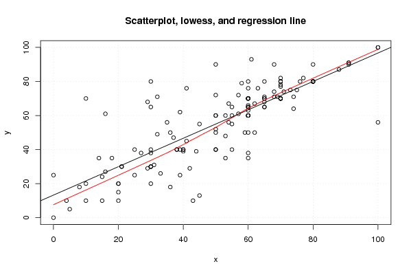
43 30 30 54 30 16 42 0 30 44 70 30 5 30 62 91 41 73 60 20 4 60 62 60 76 65 60 88 16 65 35 70 21 60 100 65 80 65 60 31 55 74 32 10 20 40 55 70 80 50 55 29 70 50 60 60 27 38 70 15 40 37 10 75 60 55 91 29 50 10 57 45 70 38 70 40 61 15 25 54 36 50 68 14 68 100 74 59 50 60 60 70 45 60 21 0 65 33 70 20 60 65 60 53 71 32 70 60 60 50 25 20 80 53 39 53 39 70 60 77 80 50 69 70 36 30 57 80 91 8 60 63 60 18 39 41 50 65 80 68 58 30 60 100 | |||||||||||||||||||||||||||||||||||||||||||||||||||||||||||||
| Dataseries Y: | |||||||||||||||||||||||||||||||||||||||||||||||||||||||||||||
10 20 40 67 38 61 29 0 30 39 70 65 5 30 50 90 45 75 76 15 10 60 67 60 80 70 70 87 27 65 56 82 30 38 56 70 80 71 50 31 40 71 71 10 20 40 55 80 80 72 60 29 70 60 63 70 38 40 80 24 40 47 70 75 60 65 91 68 90 20 61 13 80 40 70 39 93 10 25 56 18 60 74 35 71 100 64 50 40 35 60 70 55 65 30 25 80 26 78 10 70 65 80 60 74 49 70 66 65 40 40 20 90 48 25 35 40 77 70 82 80 52 71 70 50 80 72 80 91 18 70 76 65 35 62 76 50 68 80 90 79 30 60 100 | |||||||||||||||||||||||||||||||||||||||||||||||||||||||||||||
Tables (Output of Computation) | |||||||||||||||||||||||||||||||||||||||||||||||||||||||||||||
| |||||||||||||||||||||||||||||||||||||||||||||||||||||||||||||
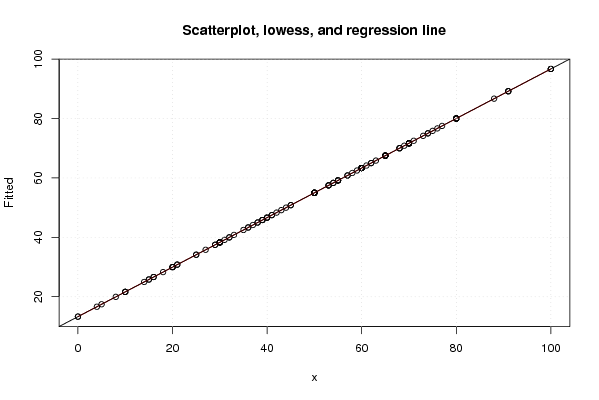
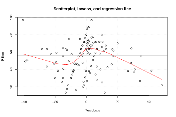
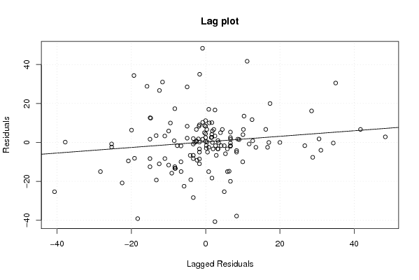
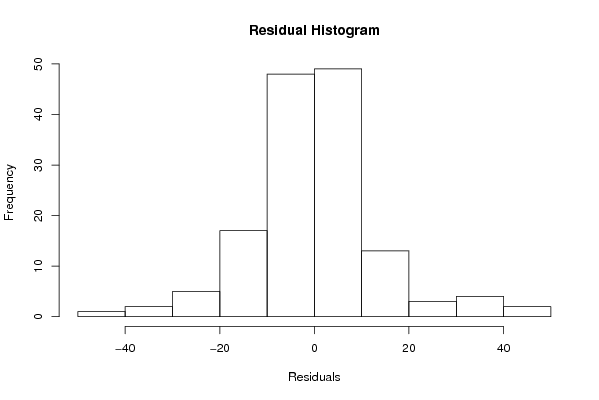
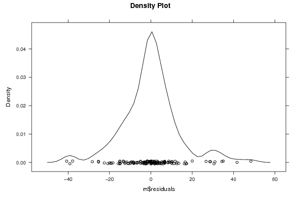
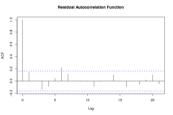
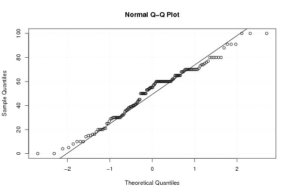
Figures (Output of Computation) | |||||||||||||||||||||||||||||||||||||||||||||||||||||||||||||
Input Parameters & R Code | |||||||||||||||||||||||||||||||||||||||||||||||||||||||||||||
| Parameters (Session): | |||||||||||||||||||||||||||||||||||||||||||||||||||||||||||||
| par1 = 0 ; | |||||||||||||||||||||||||||||||||||||||||||||||||||||||||||||
| Parameters (R input): | |||||||||||||||||||||||||||||||||||||||||||||||||||||||||||||
| par1 = 0 ; | |||||||||||||||||||||||||||||||||||||||||||||||||||||||||||||
| R code (references can be found in the software module): | |||||||||||||||||||||||||||||||||||||||||||||||||||||||||||||
par1 <- as.numeric(par1) | |||||||||||||||||||||||||||||||||||||||||||||||||||||||||||||