Free Statistics
of Irreproducible Research!
Description of Statistical Computation | |||||||||||||||||||||
|---|---|---|---|---|---|---|---|---|---|---|---|---|---|---|---|---|---|---|---|---|---|
| Author's title | |||||||||||||||||||||
| Author | *The author of this computation has been verified* | ||||||||||||||||||||
| R Software Module | rwasp_meanplot.wasp | ||||||||||||||||||||
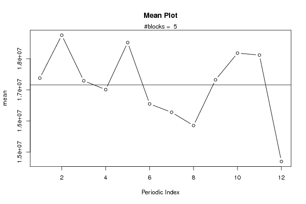
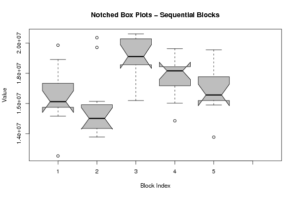
| Title produced by software | Mean Plot | ||||||||||||||||||||
| Date of computation | Mon, 15 Nov 2010 18:06:44 +0000 | ||||||||||||||||||||
| Cite this page as follows | Statistical Computations at FreeStatistics.org, Office for Research Development and Education, URL https://freestatistics.org/blog/index.php?v=date/2010/Nov/15/t1289844421gmzof5djaz71q6z.htm/, Retrieved Sun, 28 Apr 2024 10:17:10 +0000 | ||||||||||||||||||||
| Statistical Computations at FreeStatistics.org, Office for Research Development and Education, URL https://freestatistics.org/blog/index.php?pk=94972, Retrieved Sun, 28 Apr 2024 10:17:10 +0000 | |||||||||||||||||||||
| QR Codes: | |||||||||||||||||||||
|
| |||||||||||||||||||||
| Original text written by user: | |||||||||||||||||||||
| IsPrivate? | No (this computation is public) | ||||||||||||||||||||
| User-defined keywords | |||||||||||||||||||||
| Estimated Impact | 128 | ||||||||||||||||||||
Tree of Dependent Computations | |||||||||||||||||||||
| Family? (F = Feedback message, R = changed R code, M = changed R Module, P = changed Parameters, D = changed Data) | |||||||||||||||||||||
| - [Bivariate Data Series] [Bivariate dataset] [2008-01-05 23:51:08] [74be16979710d4c4e7c6647856088456] F RMPD [Mean Plot] [Colombia Coffee] [2008-01-07 13:38:24] [74be16979710d4c4e7c6647856088456] - MPD [Mean Plot] [Workshop assignme...] [2010-11-07 13:03:43] [247f085ab5b7724f755ad01dc754a3e8] - D [Mean Plot] [boxplots seasonality] [2010-11-15 18:06:44] [9d72585f2b7b60ae977d4816136e1c95] [Current] | |||||||||||||||||||||
| Feedback Forum | |||||||||||||||||||||
Post a new message | |||||||||||||||||||||
Dataset | |||||||||||||||||||||
| Dataseries X: | |||||||||||||||||||||
17681170,13 19858875,65 16997477,78 16969881,42 18908869,11 15692144,17 15159951,13 15806842,33 16007123,26 16059123,25 16189383,57 12522497,94 14733828,17 15686348,94 13779681,49 14423755,53 15290621,44 14308336,46 13855616,12 14384486,00 15638580,70 19711553,27 20359793,22 16141449,72 20056915,06 20605542,58 19325754,03 20547653,75 19211178,55 19009453,59 18746813,27 16471529,53 18957217,20 20515191,95 18374420,60 16192909,22 18147463,68 19301440,71 18344657,85 17183629,01 19629987,60 17167191,42 17428458,32 16016524,60 18466459,42 18406552,23 18174068,44 14851949,20 16260733,42 18329610,38 18003781,65 15903762,33 19554176,37 16554237,93 16198892,67 16571771,60 17535166,38 16198106,13 17487530,67 13768040,14 | |||||||||||||||||||||
Tables (Output of Computation) | |||||||||||||||||||||
| |||||||||||||||||||||
Figures (Output of Computation) | |||||||||||||||||||||
Input Parameters & R Code | |||||||||||||||||||||
| Parameters (Session): | |||||||||||||||||||||
| par1 = 12 ; | |||||||||||||||||||||
| Parameters (R input): | |||||||||||||||||||||
| par1 = 12 ; | |||||||||||||||||||||
| R code (references can be found in the software module): | |||||||||||||||||||||
par1 <- as.numeric(par1) | |||||||||||||||||||||