Repository of Reproducible Computations

Free Statistics

of Irreproducible Research!

Author's title

Author

*Unverified author*

R Software Module

rwasp_autocorrelation.wasp

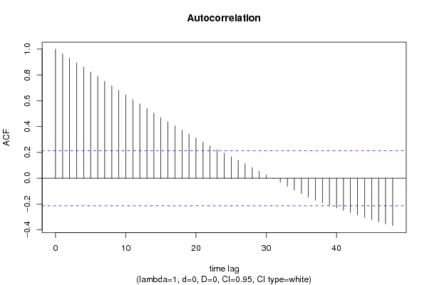
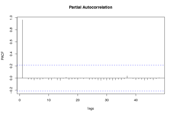
Title produced by software

(Partial) Autocorrelation Function

Date of computation

Mon, 15 Nov 2010 18:37:44 +0000

Cite this page as follows

Statistical Computations at FreeStatistics.org, Office for Research Development and Education, URL https://freestatistics.org/blog/index.php?v=date/2010/Nov/15/t1289846468y5fjrqv3qixa2n7.htm/, Retrieved Sun, 28 Apr 2024 12:54:06 +0000

Statistical Computations at FreeStatistics.org, Office for Research Development and Education, URL https://freestatistics.org/blog/index.php?pk=94995, Retrieved Sun, 28 Apr 2024 12:54:06 +0000

QR Codes:

Paste this QR Code to cite your computation.

Original text written by user:

IsPrivate?

No (this computation is public)

User-defined keywords

KDGP2W12

Estimated Impact

127

Family? (F = Feedback message, R = changed R code, M = changed R Module, P = changed Parameters, D = changed Data)

-     [] [Opgave 6bis; Opdr...] [1970-01-01 00:00:00] [07e3bd7de496d4bb901bc9a984612f8a]
- RMPD    [(Partial) Autocorrelation Function] [Opgave 6bis; Opdr...] [2010-11-15 18:37:44] [516d1a4ad1f0b8513272cbee80fe4619] [Current]

Feedback Forum

Post a new message

Dataseries X:

Download CSV

Histogram

Boxplots

Summary of computational transaction
Raw Input	view raw input (R code)
Raw Output	view raw output of R engine
Computing time	1 seconds
R Server	'Gwilym Jenkins' @ 72.249.127.135
R Framework error message	Warning: there are blank lines in the 'Data' field. Please, use NA for missing data - blank lines are simply deleted and are NOT treated as missing values.

\begin{tabular}{lllllllll}
\hline
Summary of computational transaction \tabularnewline
Raw Input & view raw input (R code)  \tabularnewline
Raw Output & view raw output of R engine  \tabularnewline
Computing time & 1 seconds \tabularnewline
R Server & 'Gwilym Jenkins' @ 72.249.127.135 \tabularnewline
R Framework error message & Warning: there are blank lines in the 'Data' field.
Please, use NA for missing data - blank lines are simply
 deleted and are NOT treated as missing values. \tabularnewline
\hline
\end{tabular}
%Source: https://freestatistics.org/blog/index.php?pk=94995&T=0

[TABLE]
[ROW][C]Summary of computational transaction[/C][/ROW]
[ROW][C]Raw Input[/C][C]view raw input (R code) [/C][/ROW]
[ROW][C]Raw Output[/C][C]view raw output of R engine [/C][/ROW]
[ROW][C]Computing time[/C][C]1 seconds[/C][/ROW]
[ROW][C]R Server[/C][C]'Gwilym Jenkins' @ 72.249.127.135[/C][/ROW]
[ROW][C]R Framework error message[/C][C]Warning: there are blank lines in the 'Data' field.
Please, use NA for missing data - blank lines are simply
 deleted and are NOT treated as missing values.[/C][/ROW]
[/TABLE]
Source: https://freestatistics.org/blog/index.php?pk=94995&T=0

Globally Unique Identifier (entire table): ba.freestatistics.org/blog/index.php?pk=94995&T=0

As an alternative you can also use a QR Code:

The GUIDs for individual cells are displayed in the table below:

Summary of computational transaction
Raw Input	view raw input (R code)
Raw Output	view raw output of R engine
Computing time	1 seconds
R Server	'Gwilym Jenkins' @ 72.249.127.135
R Framework error message	Warning: there are blank lines in the 'Data' field. Please, use NA for missing data - blank lines are simply deleted and are NOT treated as missing values.

Autocorrelation Function
Time lag k	ACF(k)	T-STAT	P-value
1	0.964014	8.8353	0
2	0.929411	8.5182	0
3	0.894691	8.2	0
4	0.859749	7.8797	0
5	0.823793	7.5502	0
6	0.788017	7.2223	0
7	0.751628	6.8888	0
8	0.715627	6.5588	0
9	0.680978	6.2413	0
10	0.645766	5.9185	0
11	0.609816	5.5891	0
12	0.575743	5.2768	1e-06
13	0.540903	4.9575	2e-06
14	0.504887	4.6274	7e-06
15	0.470164	4.3091	2.2e-05
16	0.438044	4.0147	6.4e-05
17	0.405552	3.7169	0.000181
18	0.373392	3.4222	0.000481
19	0.341788	3.1325	0.001193
20	0.310051	2.8417	0.002816
21	0.27983	2.5647	0.006052
22	0.250373	2.2947	0.012122
23	0.222596	2.0401	0.022239
24	0.194606	1.7836	0.039051
25	0.16702	1.5308	0.064793
26	0.139836	1.2816	0.101752
27	0.111908	1.0257	0.154
28	0.083209	0.7626	0.223912
29	0.054743	0.5017	0.308585
30	0.02565	0.2351	0.407357
31	-0.003399	-0.0312	0.48761
32	-0.032871	-0.3013	0.381977
33	-0.062378	-0.5717	0.284526
34	-0.09126	-0.8364	0.202648
35	-0.11984	-1.0983	0.137595
36	-0.14721	-1.3492	0.090449
37	-0.169907	-1.5572	0.061589
38	-0.190715	-1.7479	0.042065
39	-0.210215	-1.9267	0.028702
40	-0.229839	-2.1065	0.019072
41	-0.24843	-2.2769	0.012667
42	-0.266552	-2.443	0.008331
43	-0.285033	-2.6124	0.005325
44	-0.303395	-2.7807	0.003347
45	-0.320704	-2.9393	0.002123
46	-0.337987	-3.0977	0.001326
47	-0.353784	-3.2425	0.00085
48	-0.367086	-3.3644	0.000579

\begin{tabular}{lllllllll}
\hline
Autocorrelation Function \tabularnewline
Time lag k & ACF(k) & T-STAT & P-value \tabularnewline
1 & 0.964014 & 8.8353 & 0 \tabularnewline
2 & 0.929411 & 8.5182 & 0 \tabularnewline
3 & 0.894691 & 8.2 & 0 \tabularnewline
4 & 0.859749 & 7.8797 & 0 \tabularnewline
5 & 0.823793 & 7.5502 & 0 \tabularnewline
6 & 0.788017 & 7.2223 & 0 \tabularnewline
7 & 0.751628 & 6.8888 & 0 \tabularnewline
8 & 0.715627 & 6.5588 & 0 \tabularnewline
9 & 0.680978 & 6.2413 & 0 \tabularnewline
10 & 0.645766 & 5.9185 & 0 \tabularnewline
11 & 0.609816 & 5.5891 & 0 \tabularnewline
12 & 0.575743 & 5.2768 & 1e-06 \tabularnewline
13 & 0.540903 & 4.9575 & 2e-06 \tabularnewline
14 & 0.504887 & 4.6274 & 7e-06 \tabularnewline
15 & 0.470164 & 4.3091 & 2.2e-05 \tabularnewline
16 & 0.438044 & 4.0147 & 6.4e-05 \tabularnewline
17 & 0.405552 & 3.7169 & 0.000181 \tabularnewline
18 & 0.373392 & 3.4222 & 0.000481 \tabularnewline
19 & 0.341788 & 3.1325 & 0.001193 \tabularnewline
20 & 0.310051 & 2.8417 & 0.002816 \tabularnewline
21 & 0.27983 & 2.5647 & 0.006052 \tabularnewline
22 & 0.250373 & 2.2947 & 0.012122 \tabularnewline
23 & 0.222596 & 2.0401 & 0.022239 \tabularnewline
24 & 0.194606 & 1.7836 & 0.039051 \tabularnewline
25 & 0.16702 & 1.5308 & 0.064793 \tabularnewline
26 & 0.139836 & 1.2816 & 0.101752 \tabularnewline
27 & 0.111908 & 1.0257 & 0.154 \tabularnewline
28 & 0.083209 & 0.7626 & 0.223912 \tabularnewline
29 & 0.054743 & 0.5017 & 0.308585 \tabularnewline
30 & 0.02565 & 0.2351 & 0.407357 \tabularnewline
31 & -0.003399 & -0.0312 & 0.48761 \tabularnewline
32 & -0.032871 & -0.3013 & 0.381977 \tabularnewline
33 & -0.062378 & -0.5717 & 0.284526 \tabularnewline
34 & -0.09126 & -0.8364 & 0.202648 \tabularnewline
35 & -0.11984 & -1.0983 & 0.137595 \tabularnewline
36 & -0.14721 & -1.3492 & 0.090449 \tabularnewline
37 & -0.169907 & -1.5572 & 0.061589 \tabularnewline
38 & -0.190715 & -1.7479 & 0.042065 \tabularnewline
39 & -0.210215 & -1.9267 & 0.028702 \tabularnewline
40 & -0.229839 & -2.1065 & 0.019072 \tabularnewline
41 & -0.24843 & -2.2769 & 0.012667 \tabularnewline
42 & -0.266552 & -2.443 & 0.008331 \tabularnewline
43 & -0.285033 & -2.6124 & 0.005325 \tabularnewline
44 & -0.303395 & -2.7807 & 0.003347 \tabularnewline
45 & -0.320704 & -2.9393 & 0.002123 \tabularnewline
46 & -0.337987 & -3.0977 & 0.001326 \tabularnewline
47 & -0.353784 & -3.2425 & 0.00085 \tabularnewline
48 & -0.367086 & -3.3644 & 0.000579 \tabularnewline
\hline
\end{tabular}
%Source: https://freestatistics.org/blog/index.php?pk=94995&T=1

[TABLE]
[ROW][C]Autocorrelation Function[/C][/ROW]
[ROW][C]Time lag k[/C][C]ACF(k)[/C][C]T-STAT[/C][C]P-value[/C][/ROW]
[ROW][C]1[/C][C]0.964014[/C][C]8.8353[/C][C]0[/C][/ROW]
[ROW][C]2[/C][C]0.929411[/C][C]8.5182[/C][C]0[/C][/ROW]
[ROW][C]3[/C][C]0.894691[/C][C]8.2[/C][C]0[/C][/ROW]
[ROW][C]4[/C][C]0.859749[/C][C]7.8797[/C][C]0[/C][/ROW]
[ROW][C]5[/C][C]0.823793[/C][C]7.5502[/C][C]0[/C][/ROW]
[ROW][C]6[/C][C]0.788017[/C][C]7.2223[/C][C]0[/C][/ROW]
[ROW][C]7[/C][C]0.751628[/C][C]6.8888[/C][C]0[/C][/ROW]
[ROW][C]8[/C][C]0.715627[/C][C]6.5588[/C][C]0[/C][/ROW]
[ROW][C]9[/C][C]0.680978[/C][C]6.2413[/C][C]0[/C][/ROW]
[ROW][C]10[/C][C]0.645766[/C][C]5.9185[/C][C]0[/C][/ROW]
[ROW][C]11[/C][C]0.609816[/C][C]5.5891[/C][C]0[/C][/ROW]
[ROW][C]12[/C][C]0.575743[/C][C]5.2768[/C][C]1e-06[/C][/ROW]
[ROW][C]13[/C][C]0.540903[/C][C]4.9575[/C][C]2e-06[/C][/ROW]
[ROW][C]14[/C][C]0.504887[/C][C]4.6274[/C][C]7e-06[/C][/ROW]
[ROW][C]15[/C][C]0.470164[/C][C]4.3091[/C][C]2.2e-05[/C][/ROW]
[ROW][C]16[/C][C]0.438044[/C][C]4.0147[/C][C]6.4e-05[/C][/ROW]
[ROW][C]17[/C][C]0.405552[/C][C]3.7169[/C][C]0.000181[/C][/ROW]
[ROW][C]18[/C][C]0.373392[/C][C]3.4222[/C][C]0.000481[/C][/ROW]
[ROW][C]19[/C][C]0.341788[/C][C]3.1325[/C][C]0.001193[/C][/ROW]
[ROW][C]20[/C][C]0.310051[/C][C]2.8417[/C][C]0.002816[/C][/ROW]
[ROW][C]21[/C][C]0.27983[/C][C]2.5647[/C][C]0.006052[/C][/ROW]
[ROW][C]22[/C][C]0.250373[/C][C]2.2947[/C][C]0.012122[/C][/ROW]
[ROW][C]23[/C][C]0.222596[/C][C]2.0401[/C][C]0.022239[/C][/ROW]
[ROW][C]24[/C][C]0.194606[/C][C]1.7836[/C][C]0.039051[/C][/ROW]
[ROW][C]25[/C][C]0.16702[/C][C]1.5308[/C][C]0.064793[/C][/ROW]
[ROW][C]26[/C][C]0.139836[/C][C]1.2816[/C][C]0.101752[/C][/ROW]
[ROW][C]27[/C][C]0.111908[/C][C]1.0257[/C][C]0.154[/C][/ROW]
[ROW][C]28[/C][C]0.083209[/C][C]0.7626[/C][C]0.223912[/C][/ROW]
[ROW][C]29[/C][C]0.054743[/C][C]0.5017[/C][C]0.308585[/C][/ROW]
[ROW][C]30[/C][C]0.02565[/C][C]0.2351[/C][C]0.407357[/C][/ROW]
[ROW][C]31[/C][C]-0.003399[/C][C]-0.0312[/C][C]0.48761[/C][/ROW]
[ROW][C]32[/C][C]-0.032871[/C][C]-0.3013[/C][C]0.381977[/C][/ROW]
[ROW][C]33[/C][C]-0.062378[/C][C]-0.5717[/C][C]0.284526[/C][/ROW]
[ROW][C]34[/C][C]-0.09126[/C][C]-0.8364[/C][C]0.202648[/C][/ROW]
[ROW][C]35[/C][C]-0.11984[/C][C]-1.0983[/C][C]0.137595[/C][/ROW]
[ROW][C]36[/C][C]-0.14721[/C][C]-1.3492[/C][C]0.090449[/C][/ROW]
[ROW][C]37[/C][C]-0.169907[/C][C]-1.5572[/C][C]0.061589[/C][/ROW]
[ROW][C]38[/C][C]-0.190715[/C][C]-1.7479[/C][C]0.042065[/C][/ROW]
[ROW][C]39[/C][C]-0.210215[/C][C]-1.9267[/C][C]0.028702[/C][/ROW]
[ROW][C]40[/C][C]-0.229839[/C][C]-2.1065[/C][C]0.019072[/C][/ROW]
[ROW][C]41[/C][C]-0.24843[/C][C]-2.2769[/C][C]0.012667[/C][/ROW]
[ROW][C]42[/C][C]-0.266552[/C][C]-2.443[/C][C]0.008331[/C][/ROW]
[ROW][C]43[/C][C]-0.285033[/C][C]-2.6124[/C][C]0.005325[/C][/ROW]
[ROW][C]44[/C][C]-0.303395[/C][C]-2.7807[/C][C]0.003347[/C][/ROW]
[ROW][C]45[/C][C]-0.320704[/C][C]-2.9393[/C][C]0.002123[/C][/ROW]
[ROW][C]46[/C][C]-0.337987[/C][C]-3.0977[/C][C]0.001326[/C][/ROW]
[ROW][C]47[/C][C]-0.353784[/C][C]-3.2425[/C][C]0.00085[/C][/ROW]
[ROW][C]48[/C][C]-0.367086[/C][C]-3.3644[/C][C]0.000579[/C][/ROW]
[/TABLE]
Source: https://freestatistics.org/blog/index.php?pk=94995&T=1

Globally Unique Identifier (entire table): ba.freestatistics.org/blog/index.php?pk=94995&T=1

As an alternative you can also use a QR Code:

The GUIDs for individual cells are displayed in the table below:

Autocorrelation Function
Time lag k	ACF(k)	T-STAT	P-value
1	0.964014	8.8353	0
2	0.929411	8.5182	0
3	0.894691	8.2	0
4	0.859749	7.8797	0
5	0.823793	7.5502	0
6	0.788017	7.2223	0
7	0.751628	6.8888	0
8	0.715627	6.5588	0
9	0.680978	6.2413	0
10	0.645766	5.9185	0
11	0.609816	5.5891	0
12	0.575743	5.2768	1e-06
13	0.540903	4.9575	2e-06
14	0.504887	4.6274	7e-06
15	0.470164	4.3091	2.2e-05
16	0.438044	4.0147	6.4e-05
17	0.405552	3.7169	0.000181
18	0.373392	3.4222	0.000481
19	0.341788	3.1325	0.001193
20	0.310051	2.8417	0.002816
21	0.27983	2.5647	0.006052
22	0.250373	2.2947	0.012122
23	0.222596	2.0401	0.022239
24	0.194606	1.7836	0.039051
25	0.16702	1.5308	0.064793
26	0.139836	1.2816	0.101752
27	0.111908	1.0257	0.154
28	0.083209	0.7626	0.223912
29	0.054743	0.5017	0.308585
30	0.02565	0.2351	0.407357
31	-0.003399	-0.0312	0.48761
32	-0.032871	-0.3013	0.381977
33	-0.062378	-0.5717	0.284526
34	-0.09126	-0.8364	0.202648
35	-0.11984	-1.0983	0.137595
36	-0.14721	-1.3492	0.090449
37	-0.169907	-1.5572	0.061589
38	-0.190715	-1.7479	0.042065
39	-0.210215	-1.9267	0.028702
40	-0.229839	-2.1065	0.019072
41	-0.24843	-2.2769	0.012667
42	-0.266552	-2.443	0.008331
43	-0.285033	-2.6124	0.005325
44	-0.303395	-2.7807	0.003347
45	-0.320704	-2.9393	0.002123
46	-0.337987	-3.0977	0.001326
47	-0.353784	-3.2425	0.00085
48	-0.367086	-3.3644	0.000579

Partial Autocorrelation Function
Time lag k	PACF(k)	T-STAT	P-value
1	0.964014	8.8353	0
2	0.001238	0.0113	0.495486
3	-0.019222	-0.1762	0.43029
4	-0.021516	-0.1972	0.422075
5	-0.033269	-0.3049	0.380594
6	-0.0177	-0.1622	0.435761
7	-0.028579	-0.2619	0.397009
8	-0.015524	-0.1423	0.443602
9	-0.001383	-0.0127	0.494959
10	-0.027909	-0.2558	0.39937
11	-0.031985	-0.2931	0.385067
12	0.003674	0.0337	0.486611
13	-0.031924	-0.2926	0.385278
14	-0.039567	-0.3626	0.358894
15	-0.006264	-0.0574	0.477178
16	0.0138	0.1265	0.449828
17	-0.025499	-0.2337	0.407892
18	-0.019253	-0.1765	0.430181
19	-0.016012	-0.1468	0.441839
20	-0.024993	-0.2291	0.409688
21	-0.003782	-0.0347	0.486217
22	-0.013782	-0.1263	0.449891
23	0.002389	0.0219	0.49129
24	-0.024735	-0.2267	0.410603
25	-0.020944	-0.192	0.424119
26	-0.017953	-0.1645	0.434848
27	-0.034053	-0.3121	0.377869
28	-0.038931	-0.3568	0.361065
29	-0.024618	-0.2256	0.41102
30	-0.034514	-0.3163	0.37627
31	-0.027268	-0.2499	0.401631
32	-0.035496	-0.3253	0.372872
33	-0.031183	-0.2858	0.387869
34	-0.021728	-0.1991	0.421316
35	-0.028886	-0.2647	0.395928
36	-0.014334	-0.1314	0.447899
37	0.037229	0.3412	0.366898
38	0.001014	0.0093	0.496303
39	-0.009469	-0.0868	0.465524
40	-0.028882	-0.2647	0.395941
41	-0.015599	-0.143	0.443331
42	-0.023175	-0.2124	0.416154
43	-0.035676	-0.327	0.37225
44	-0.028336	-0.2597	0.397864
45	-0.014214	-0.1303	0.44833
46	-0.031116	-0.2852	0.388103
47	-0.012654	-0.116	0.453975
48	0.006317	0.0579	0.476983

\begin{tabular}{lllllllll}
\hline
Partial Autocorrelation Function \tabularnewline
Time lag k & PACF(k) & T-STAT & P-value \tabularnewline
1 & 0.964014 & 8.8353 & 0 \tabularnewline
2 & 0.001238 & 0.0113 & 0.495486 \tabularnewline
3 & -0.019222 & -0.1762 & 0.43029 \tabularnewline
4 & -0.021516 & -0.1972 & 0.422075 \tabularnewline
5 & -0.033269 & -0.3049 & 0.380594 \tabularnewline
6 & -0.0177 & -0.1622 & 0.435761 \tabularnewline
7 & -0.028579 & -0.2619 & 0.397009 \tabularnewline
8 & -0.015524 & -0.1423 & 0.443602 \tabularnewline
9 & -0.001383 & -0.0127 & 0.494959 \tabularnewline
10 & -0.027909 & -0.2558 & 0.39937 \tabularnewline
11 & -0.031985 & -0.2931 & 0.385067 \tabularnewline
12 & 0.003674 & 0.0337 & 0.486611 \tabularnewline
13 & -0.031924 & -0.2926 & 0.385278 \tabularnewline
14 & -0.039567 & -0.3626 & 0.358894 \tabularnewline
15 & -0.006264 & -0.0574 & 0.477178 \tabularnewline
16 & 0.0138 & 0.1265 & 0.449828 \tabularnewline
17 & -0.025499 & -0.2337 & 0.407892 \tabularnewline
18 & -0.019253 & -0.1765 & 0.430181 \tabularnewline
19 & -0.016012 & -0.1468 & 0.441839 \tabularnewline
20 & -0.024993 & -0.2291 & 0.409688 \tabularnewline
21 & -0.003782 & -0.0347 & 0.486217 \tabularnewline
22 & -0.013782 & -0.1263 & 0.449891 \tabularnewline
23 & 0.002389 & 0.0219 & 0.49129 \tabularnewline
24 & -0.024735 & -0.2267 & 0.410603 \tabularnewline
25 & -0.020944 & -0.192 & 0.424119 \tabularnewline
26 & -0.017953 & -0.1645 & 0.434848 \tabularnewline
27 & -0.034053 & -0.3121 & 0.377869 \tabularnewline
28 & -0.038931 & -0.3568 & 0.361065 \tabularnewline
29 & -0.024618 & -0.2256 & 0.41102 \tabularnewline
30 & -0.034514 & -0.3163 & 0.37627 \tabularnewline
31 & -0.027268 & -0.2499 & 0.401631 \tabularnewline
32 & -0.035496 & -0.3253 & 0.372872 \tabularnewline
33 & -0.031183 & -0.2858 & 0.387869 \tabularnewline
34 & -0.021728 & -0.1991 & 0.421316 \tabularnewline
35 & -0.028886 & -0.2647 & 0.395928 \tabularnewline
36 & -0.014334 & -0.1314 & 0.447899 \tabularnewline
37 & 0.037229 & 0.3412 & 0.366898 \tabularnewline
38 & 0.001014 & 0.0093 & 0.496303 \tabularnewline
39 & -0.009469 & -0.0868 & 0.465524 \tabularnewline
40 & -0.028882 & -0.2647 & 0.395941 \tabularnewline
41 & -0.015599 & -0.143 & 0.443331 \tabularnewline
42 & -0.023175 & -0.2124 & 0.416154 \tabularnewline
43 & -0.035676 & -0.327 & 0.37225 \tabularnewline
44 & -0.028336 & -0.2597 & 0.397864 \tabularnewline
45 & -0.014214 & -0.1303 & 0.44833 \tabularnewline
46 & -0.031116 & -0.2852 & 0.388103 \tabularnewline
47 & -0.012654 & -0.116 & 0.453975 \tabularnewline
48 & 0.006317 & 0.0579 & 0.476983 \tabularnewline
\hline
\end{tabular}
%Source: https://freestatistics.org/blog/index.php?pk=94995&T=2

[TABLE]
[ROW][C]Partial Autocorrelation Function[/C][/ROW]
[ROW][C]Time lag k[/C][C]PACF(k)[/C][C]T-STAT[/C][C]P-value[/C][/ROW]
[ROW][C]1[/C][C]0.964014[/C][C]8.8353[/C][C]0[/C][/ROW]
[ROW][C]2[/C][C]0.001238[/C][C]0.0113[/C][C]0.495486[/C][/ROW]
[ROW][C]3[/C][C]-0.019222[/C][C]-0.1762[/C][C]0.43029[/C][/ROW]
[ROW][C]4[/C][C]-0.021516[/C][C]-0.1972[/C][C]0.422075[/C][/ROW]
[ROW][C]5[/C][C]-0.033269[/C][C]-0.3049[/C][C]0.380594[/C][/ROW]
[ROW][C]6[/C][C]-0.0177[/C][C]-0.1622[/C][C]0.435761[/C][/ROW]
[ROW][C]7[/C][C]-0.028579[/C][C]-0.2619[/C][C]0.397009[/C][/ROW]
[ROW][C]8[/C][C]-0.015524[/C][C]-0.1423[/C][C]0.443602[/C][/ROW]
[ROW][C]9[/C][C]-0.001383[/C][C]-0.0127[/C][C]0.494959[/C][/ROW]
[ROW][C]10[/C][C]-0.027909[/C][C]-0.2558[/C][C]0.39937[/C][/ROW]
[ROW][C]11[/C][C]-0.031985[/C][C]-0.2931[/C][C]0.385067[/C][/ROW]
[ROW][C]12[/C][C]0.003674[/C][C]0.0337[/C][C]0.486611[/C][/ROW]
[ROW][C]13[/C][C]-0.031924[/C][C]-0.2926[/C][C]0.385278[/C][/ROW]
[ROW][C]14[/C][C]-0.039567[/C][C]-0.3626[/C][C]0.358894[/C][/ROW]
[ROW][C]15[/C][C]-0.006264[/C][C]-0.0574[/C][C]0.477178[/C][/ROW]
[ROW][C]16[/C][C]0.0138[/C][C]0.1265[/C][C]0.449828[/C][/ROW]
[ROW][C]17[/C][C]-0.025499[/C][C]-0.2337[/C][C]0.407892[/C][/ROW]
[ROW][C]18[/C][C]-0.019253[/C][C]-0.1765[/C][C]0.430181[/C][/ROW]
[ROW][C]19[/C][C]-0.016012[/C][C]-0.1468[/C][C]0.441839[/C][/ROW]
[ROW][C]20[/C][C]-0.024993[/C][C]-0.2291[/C][C]0.409688[/C][/ROW]
[ROW][C]21[/C][C]-0.003782[/C][C]-0.0347[/C][C]0.486217[/C][/ROW]
[ROW][C]22[/C][C]-0.013782[/C][C]-0.1263[/C][C]0.449891[/C][/ROW]
[ROW][C]23[/C][C]0.002389[/C][C]0.0219[/C][C]0.49129[/C][/ROW]
[ROW][C]24[/C][C]-0.024735[/C][C]-0.2267[/C][C]0.410603[/C][/ROW]
[ROW][C]25[/C][C]-0.020944[/C][C]-0.192[/C][C]0.424119[/C][/ROW]
[ROW][C]26[/C][C]-0.017953[/C][C]-0.1645[/C][C]0.434848[/C][/ROW]
[ROW][C]27[/C][C]-0.034053[/C][C]-0.3121[/C][C]0.377869[/C][/ROW]
[ROW][C]28[/C][C]-0.038931[/C][C]-0.3568[/C][C]0.361065[/C][/ROW]
[ROW][C]29[/C][C]-0.024618[/C][C]-0.2256[/C][C]0.41102[/C][/ROW]
[ROW][C]30[/C][C]-0.034514[/C][C]-0.3163[/C][C]0.37627[/C][/ROW]
[ROW][C]31[/C][C]-0.027268[/C][C]-0.2499[/C][C]0.401631[/C][/ROW]
[ROW][C]32[/C][C]-0.035496[/C][C]-0.3253[/C][C]0.372872[/C][/ROW]
[ROW][C]33[/C][C]-0.031183[/C][C]-0.2858[/C][C]0.387869[/C][/ROW]
[ROW][C]34[/C][C]-0.021728[/C][C]-0.1991[/C][C]0.421316[/C][/ROW]
[ROW][C]35[/C][C]-0.028886[/C][C]-0.2647[/C][C]0.395928[/C][/ROW]
[ROW][C]36[/C][C]-0.014334[/C][C]-0.1314[/C][C]0.447899[/C][/ROW]
[ROW][C]37[/C][C]0.037229[/C][C]0.3412[/C][C]0.366898[/C][/ROW]
[ROW][C]38[/C][C]0.001014[/C][C]0.0093[/C][C]0.496303[/C][/ROW]
[ROW][C]39[/C][C]-0.009469[/C][C]-0.0868[/C][C]0.465524[/C][/ROW]
[ROW][C]40[/C][C]-0.028882[/C][C]-0.2647[/C][C]0.395941[/C][/ROW]
[ROW][C]41[/C][C]-0.015599[/C][C]-0.143[/C][C]0.443331[/C][/ROW]
[ROW][C]42[/C][C]-0.023175[/C][C]-0.2124[/C][C]0.416154[/C][/ROW]
[ROW][C]43[/C][C]-0.035676[/C][C]-0.327[/C][C]0.37225[/C][/ROW]
[ROW][C]44[/C][C]-0.028336[/C][C]-0.2597[/C][C]0.397864[/C][/ROW]
[ROW][C]45[/C][C]-0.014214[/C][C]-0.1303[/C][C]0.44833[/C][/ROW]
[ROW][C]46[/C][C]-0.031116[/C][C]-0.2852[/C][C]0.388103[/C][/ROW]
[ROW][C]47[/C][C]-0.012654[/C][C]-0.116[/C][C]0.453975[/C][/ROW]
[ROW][C]48[/C][C]0.006317[/C][C]0.0579[/C][C]0.476983[/C][/ROW]
[/TABLE]
Source: https://freestatistics.org/blog/index.php?pk=94995&T=2

Globally Unique Identifier (entire table): ba.freestatistics.org/blog/index.php?pk=94995&T=2

As an alternative you can also use a QR Code:

The GUIDs for individual cells are displayed in the table below:

Partial Autocorrelation Function
Time lag k	PACF(k)	T-STAT	P-value
1	0.964014	8.8353	0
2	0.001238	0.0113	0.495486
3	-0.019222	-0.1762	0.43029
4	-0.021516	-0.1972	0.422075
5	-0.033269	-0.3049	0.380594
6	-0.0177	-0.1622	0.435761
7	-0.028579	-0.2619	0.397009
8	-0.015524	-0.1423	0.443602
9	-0.001383	-0.0127	0.494959
10	-0.027909	-0.2558	0.39937
11	-0.031985	-0.2931	0.385067
12	0.003674	0.0337	0.486611
13	-0.031924	-0.2926	0.385278
14	-0.039567	-0.3626	0.358894
15	-0.006264	-0.0574	0.477178
16	0.0138	0.1265	0.449828
17	-0.025499	-0.2337	0.407892
18	-0.019253	-0.1765	0.430181
19	-0.016012	-0.1468	0.441839
20	-0.024993	-0.2291	0.409688
21	-0.003782	-0.0347	0.486217
22	-0.013782	-0.1263	0.449891
23	0.002389	0.0219	0.49129
24	-0.024735	-0.2267	0.410603
25	-0.020944	-0.192	0.424119
26	-0.017953	-0.1645	0.434848
27	-0.034053	-0.3121	0.377869
28	-0.038931	-0.3568	0.361065
29	-0.024618	-0.2256	0.41102
30	-0.034514	-0.3163	0.37627
31	-0.027268	-0.2499	0.401631
32	-0.035496	-0.3253	0.372872
33	-0.031183	-0.2858	0.387869
34	-0.021728	-0.1991	0.421316
35	-0.028886	-0.2647	0.395928
36	-0.014334	-0.1314	0.447899
37	0.037229	0.3412	0.366898
38	0.001014	0.0093	0.496303
39	-0.009469	-0.0868	0.465524
40	-0.028882	-0.2647	0.395941
41	-0.015599	-0.143	0.443331
42	-0.023175	-0.2124	0.416154
43	-0.035676	-0.327	0.37225
44	-0.028336	-0.2597	0.397864
45	-0.014214	-0.1303	0.44833
46	-0.031116	-0.2852	0.388103
47	-0.012654	-0.116	0.453975
48	0.006317	0.0579	0.476983

Figure 1

PNG link

Postscript link

PDF link

Figure 2

PNG link

Postscript link

PDF link

Parameters (Session):

par1 = 48 ; par2 = 1 ; par3 = 0 ; par4 = 0 ; par5 = 12 ; par6 = White Noise ; par7 = 0.95 ;

Parameters (R input):

par1 = 48 ; par2 = 1 ; par3 = 0 ; par4 = 0 ; par5 = 12 ; par6 = White Noise ; par7 = 0.95 ;

R code (references can be found in the software module):

if (par1 == 'Default') {
par1 = 10*log10(length(x))
} else {
par1 <- as.numeric(par1)
}
par2 <- as.numeric(par2)
par3 <- as.numeric(par3)
par4 <- as.numeric(par4)
par5 <- as.numeric(par5)
if (par6 == 'White Noise') par6 <- 'white' else par6 <- 'ma'
par7 <- as.numeric(par7)
if (par2 == 0) {
x <- log(x)
} else {
x <- (x ^ par2 - 1) / par2
}
if (par3 > 0) x <- diff(x,lag=1,difference=par3)
if (par4 > 0) x <- diff(x,lag=par5,difference=par4)
bitmap(file='pic1.png')
racf <- acf(x, par1, main='Autocorrelation', xlab='time lag', ylab='ACF', ci.type=par6, ci=par7, sub=paste('(lambda=',par2,', d=',par3,', D=',par4,', CI=', par7, ', CI type=',par6,')',sep=''))
dev.off()
bitmap(file='pic2.png')
rpacf <- pacf(x,par1,main='Partial Autocorrelation',xlab='lags',ylab='PACF')
dev.off()
(myacf <- c(racf$acf))
(mypacf <- c(rpacf$acf))
lengthx <- length(x)
sqrtn <- sqrt(lengthx)
load(file='createtable')
a<-table.start()
a<-table.row.start(a)
a<-table.element(a,'Autocorrelation Function',4,TRUE)
a<-table.row.end(a)
a<-table.row.start(a)
a<-table.element(a,'Time lag k',header=TRUE)
a<-table.element(a,hyperlink('basics.htm','ACF(k)','click here for more information about the Autocorrelation Function'),header=TRUE)
a<-table.element(a,'T-STAT',header=TRUE)
a<-table.element(a,'P-value',header=TRUE)
a<-table.row.end(a)
for (i in 2:(par1+1)) {
a<-table.row.start(a)
a<-table.element(a,i-1,header=TRUE)
a<-table.element(a,round(myacf[i],6))
mytstat <- myacf[i]*sqrtn
a<-table.element(a,round(mytstat,4))
a<-table.element(a,round(1-pt(abs(mytstat),lengthx),6))
a<-table.row.end(a)
}
a<-table.end(a)
table.save(a,file='mytable.tab')
a<-table.start()
a<-table.row.start(a)
a<-table.element(a,'Partial Autocorrelation Function',4,TRUE)
a<-table.row.end(a)
a<-table.row.start(a)
a<-table.element(a,'Time lag k',header=TRUE)
a<-table.element(a,hyperlink('basics.htm','PACF(k)','click here for more information about the Partial Autocorrelation Function'),header=TRUE)
a<-table.element(a,'T-STAT',header=TRUE)
a<-table.element(a,'P-value',header=TRUE)
a<-table.row.end(a)
for (i in 1:par1) {
a<-table.row.start(a)
a<-table.element(a,i,header=TRUE)
a<-table.element(a,round(mypacf[i],6))
mytstat <- mypacf[i]*sqrtn
a<-table.element(a,round(mytstat,4))
a<-table.element(a,round(1-pt(abs(mytstat),lengthx),6))
a<-table.row.end(a)
}
a<-table.end(a)
table.save(a,file='mytable1.tab')

Free Statistics

Description of Statistical Computation

Tree of Dependent Computations

Dataset

Tables (Output of Computation)

Figures (Output of Computation)

Input Parameters & R Code