Free Statistics
of Irreproducible Research!
Description of Statistical Computation | |||||||||||||||||||||||||||||||||||||||||||||||||||||||||||||
|---|---|---|---|---|---|---|---|---|---|---|---|---|---|---|---|---|---|---|---|---|---|---|---|---|---|---|---|---|---|---|---|---|---|---|---|---|---|---|---|---|---|---|---|---|---|---|---|---|---|---|---|---|---|---|---|---|---|---|---|---|---|
| Author's title | |||||||||||||||||||||||||||||||||||||||||||||||||||||||||||||
| Author | *The author of this computation has been verified* | ||||||||||||||||||||||||||||||||||||||||||||||||||||||||||||
| R Software Module | rwasp_linear_regression.wasp | ||||||||||||||||||||||||||||||||||||||||||||||||||||||||||||
| Title produced by software | Linear Regression Graphical Model Validation | ||||||||||||||||||||||||||||||||||||||||||||||||||||||||||||
| Date of computation | Mon, 15 Nov 2010 20:21:25 +0000 | ||||||||||||||||||||||||||||||||||||||||||||||||||||||||||||
| Cite this page as follows | Statistical Computations at FreeStatistics.org, Office for Research Development and Education, URL https://freestatistics.org/blog/index.php?v=date/2010/Nov/15/t12898524097qve8ggpie0yyh5.htm/, Retrieved Sat, 27 Apr 2024 18:07:50 +0000 | ||||||||||||||||||||||||||||||||||||||||||||||||||||||||||||
| Statistical Computations at FreeStatistics.org, Office for Research Development and Education, URL https://freestatistics.org/blog/index.php?pk=95047, Retrieved Sat, 27 Apr 2024 18:07:50 +0000 | |||||||||||||||||||||||||||||||||||||||||||||||||||||||||||||
| QR Codes: | |||||||||||||||||||||||||||||||||||||||||||||||||||||||||||||
|
| |||||||||||||||||||||||||||||||||||||||||||||||||||||||||||||
| Original text written by user: | |||||||||||||||||||||||||||||||||||||||||||||||||||||||||||||
| IsPrivate? | No (this computation is public) | ||||||||||||||||||||||||||||||||||||||||||||||||||||||||||||
| User-defined keywords | |||||||||||||||||||||||||||||||||||||||||||||||||||||||||||||
| Estimated Impact | 158 | ||||||||||||||||||||||||||||||||||||||||||||||||||||||||||||
Tree of Dependent Computations | |||||||||||||||||||||||||||||||||||||||||||||||||||||||||||||
| Family? (F = Feedback message, R = changed R code, M = changed R Module, P = changed Parameters, D = changed Data) | |||||||||||||||||||||||||||||||||||||||||||||||||||||||||||||
| - [Paired and Unpaired Two Samples Tests about the Mean] [Dagelijkse omzet ...] [2010-10-25 11:22:12] [b98453cac15ba1066b407e146608df68] - PD [Paired and Unpaired Two Samples Tests about the Mean] [question 5 T] [2010-10-29 12:27:53] [c1605865773cc027e55b238d879a644c] - D [Paired and Unpaired Two Samples Tests about the Mean] [] [2010-11-01 09:41:08] [22937c5b58c14f6c22964f32d64ff823] F [Paired and Unpaired Two Samples Tests about the Mean] [Workshop 5 Questi...] [2010-11-01 15:47:21] [945bcebba5e7ac34a41d6888338a1ba9] - [Paired and Unpaired Two Samples Tests about the Mean] [] [2010-11-02 14:45:56] [5278e0a58c5de897b31ce79607e774d7] - RMPD [Linear Regression Graphical Model Validation] [Mini-Tutorial Hyp...] [2010-11-15 20:21:25] [67e3c2d70de1dbb070b545ca6c893d5e] [Current] - D [Linear Regression Graphical Model Validation] [WS6 Minitutorial H1] [2010-11-15 20:32:21] [07a238a5afc23eb944f8545182f29d5a] - R D [Linear Regression Graphical Model Validation] [ws 6 -minitutorial] [2010-11-16 17:45:24] [4eaa304e6a28c475ba490fccf4c01ad3] | |||||||||||||||||||||||||||||||||||||||||||||||||||||||||||||
| Feedback Forum | |||||||||||||||||||||||||||||||||||||||||||||||||||||||||||||
Post a new message | |||||||||||||||||||||||||||||||||||||||||||||||||||||||||||||
Dataset | |||||||||||||||||||||||||||||||||||||||||||||||||||||||||||||
| Dataseries X: | |||||||||||||||||||||||||||||||||||||||||||||||||||||||||||||
24 25 30 19 22 22 25 23 17 21 19 19 15 16 23 27 22 14 22 23 23 21 19 18 20 23 25 19 24 22 25 26 29 32 25 29 28 17 28 29 26 25 14 25 26 20 18 32 25 25 23 21 20 15 30 24 26 24 22 14 24 24 24 24 19 31 22 27 19 25 20 21 27 23 25 20 21 22 23 25 25 17 19 25 19 20 26 23 27 17 17 19 17 22 21 32 21 21 18 18 23 19 20 21 20 17 18 19 22 15 14 18 24 35 29 21 25 20 22 13 26 17 25 20 19 21 22 24 21 26 24 16 23 18 16 26 19 21 21 22 23 29 21 21 23 27 25 21 10 20 26 24 29 19 24 19 24 22 17 | |||||||||||||||||||||||||||||||||||||||||||||||||||||||||||||
| Dataseries Y: | |||||||||||||||||||||||||||||||||||||||||||||||||||||||||||||
23 15 25 18 21 19 15 22 19 20 26 26 21 18 19 19 18 19 24 28 20 29 27 18 19 24 21 22 25 19 15 34 23 19 26 15 15 17 30 19 28 23 23 21 18 19 24 15 20 24 9 20 20 10 44 20 20 20 11 21 21 19 21 17 16 14 19 21 16 19 19 16 24 29 21 20 19 23 18 19 23 19 21 26 13 23 16 17 30 19 22 14 14 21 21 33 23 30 19 21 25 18 29 25 21 16 17 23 26 18 19 28 20 29 19 18 25 15 24 12 11 19 25 12 15 25 14 19 23 19 24 20 16 13 20 30 18 22 21 25 18 25 44 12 28 17 26 18 21 24 20 24 28 20 33 19 19 25 35 | |||||||||||||||||||||||||||||||||||||||||||||||||||||||||||||
Tables (Output of Computation) | |||||||||||||||||||||||||||||||||||||||||||||||||||||||||||||
| |||||||||||||||||||||||||||||||||||||||||||||||||||||||||||||
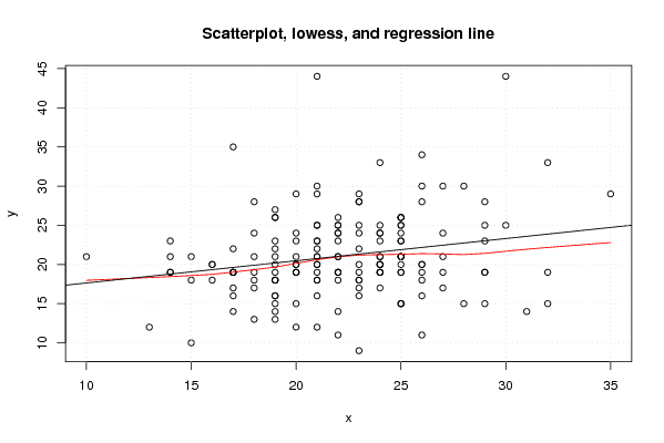
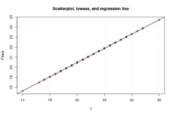
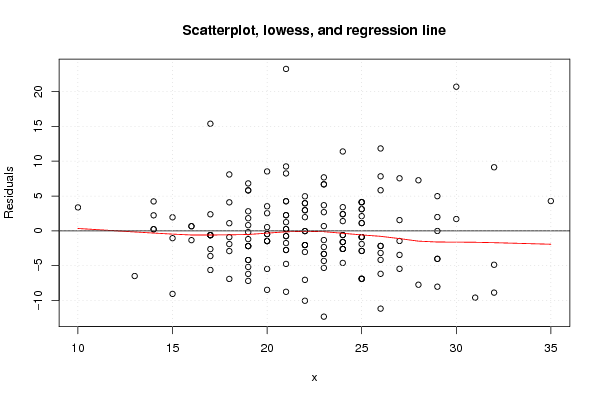
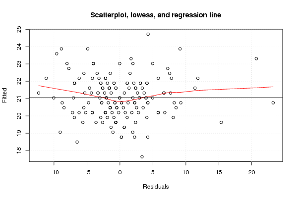
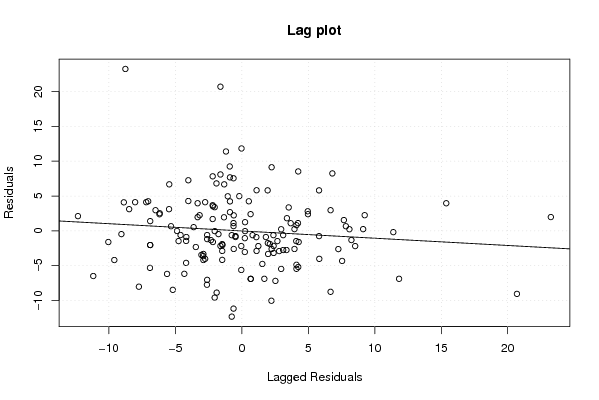
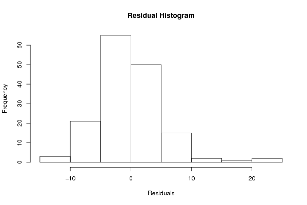
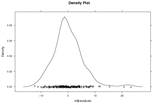
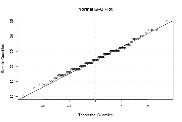
Figures (Output of Computation) | |||||||||||||||||||||||||||||||||||||||||||||||||||||||||||||
Input Parameters & R Code | |||||||||||||||||||||||||||||||||||||||||||||||||||||||||||||
| Parameters (Session): | |||||||||||||||||||||||||||||||||||||||||||||||||||||||||||||
| par1 = 0 ; | |||||||||||||||||||||||||||||||||||||||||||||||||||||||||||||
| Parameters (R input): | |||||||||||||||||||||||||||||||||||||||||||||||||||||||||||||
| par1 = 0 ; | |||||||||||||||||||||||||||||||||||||||||||||||||||||||||||||
| R code (references can be found in the software module): | |||||||||||||||||||||||||||||||||||||||||||||||||||||||||||||
par1 <- as.numeric(par1) | |||||||||||||||||||||||||||||||||||||||||||||||||||||||||||||