Repository of Reproducible Computations

Free Statistics

of Irreproducible Research!

Author's title

Author

*The author of this computation has been verified*

R Software Module

rwasp_autocorrelation.wasp

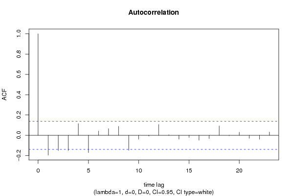
Title produced by software

(Partial) Autocorrelation Function

Date of computation

Mon, 22 Nov 2010 14:48:14 +0000

Cite this page as follows

Statistical Computations at FreeStatistics.org, Office for Research Development and Education, URL https://freestatistics.org/blog/index.php?v=date/2010/Nov/22/t1290437173a0cmb5zlmmi5xm4.htm/, Retrieved Fri, 03 May 2024 16:03:08 +0000

Statistical Computations at FreeStatistics.org, Office for Research Development and Education, URL https://freestatistics.org/blog/index.php?pk=98549, Retrieved Fri, 03 May 2024 16:03:08 +0000

QR Codes:

Paste this QR Code to cite your computation.

Original text written by user:

IsPrivate?

No (this computation is public)

User-defined keywords

Estimated Impact

123

Family? (F = Feedback message, R = changed R code, M = changed R Module, P = changed Parameters, D = changed Data)

-       [(Partial) Autocorrelation Function] [] [2010-11-22 14:48:14] [9b9a58c480cb5dafe4bfceb51e1cfd12] [Current]

Feedback Forum

Post a new message

Dataseries X:

Download CSV

Histogram

Boxplots

4.5297099404706E-14
4.5297099404706E-14
4.5297099404706E-14
4.5297099404706E-14
4.5297099404706E-14
4.5297099404706E-14
0.023924586085245
0
0
0
0
0
0
0
0
0
0
-0.0239245860852
4.5297099404706E-14
4.5297099404706E-14
0.023924586085245
0
0
0
0
-0.0239245860852
4.5297099404706E-14
4.5297099404706E-14
0.023924586085245
0
0
0
0
-0.0239245860852
4.5297099404706E-14
4.5297099404706E-14
4.5297099404706E-14
4.5297099404706E-14
4.5297099404706E-14
0.023924586085245
0
0
0
0
0
0
-0.0239245860852
4.5297099404706E-14
4.5297099404706E-14
0.023924586085245
0
0
0
-0.0239245860852
4.5297099404706E-14
0.023924586085245
0
0
0
0
-0.0239245860852
4.5297099404706E-14
4.5297099404706E-14
4.5297099404706E-14
4.5297099404706E-14
4.5297099404706E-14
4.5297099404706E-14
4.5297099404706E-14
4.5297099404706E-14
4.5297099404706E-14
4.5297099404706E-14
4.5297099404706E-14
4.5297099404706E-14
4.5297099404706E-14
0.023924586085245
0
-0.0239245860852
4.5297099404706E-14
0.023924586085245
0
0
-0.0239245860852
4.5297099404706E-14
4.5297099404706E-14
4.5297099404706E-14
4.5297099404706E-14
0.023924586085245
0
-0.0239245860852
4.5297099404706E-14
4.5297099404706E-14
0.023924586085245
0
0
-0.0239245860852
4.5297099404706E-14
4.5297099404706E-14
4.5297099404706E-14
0.023924586085245
0
-0.0239245860852
4.5297099404706E-14
0.023924586085245
0
0
0
0
0
0
0
0
0.011083236878
-0.025026669717283
-3.5971225997855E-14
-3.5971225997855E-14
-3.5971225997855E-14
0.025026669717264
1.7763568394003E-14
1.7763568394003E-14
1.7763568394003E-14
1.7763568394003E-14
1.7763568394003E-14
1.7763568394003E-14
1.7763568394003E-14
1.7763568394003E-14
1.7763568394003E-14
1.7763568394003E-14
1.7763568394003E-14
1.7763568394003E-14
1.7763568394003E-14
1.7763568394003E-14
1.7763568394003E-14
-0.025026669717283
-3.5971225997855E-14
-3.5971225997855E-14
-3.5971225997855E-14
-3.5971225997855E-14
0.025026669717264
-0.025026669717283
0.025026669717264
1.7763568394003E-14
1.7763568394003E-14
1.7763568394003E-14
1.7763568394003E-14
1.7763568394003E-14
1.7763568394003E-14
1.7763568394003E-14
-0.025026669717283
0.025026669717264
1.7763568394003E-14
1.7763568394003E-14
1.7763568394003E-14
1.7763568394003E-14
1.7763568394003E-14
-0.025026669717283
-3.5971225997855E-14
-3.5971225997855E-14
-3.5971225997855E-14
-3.5971225997855E-14
-3.5971225997855E-14
-3.5971225997855E-14
0.025026669717264
1.7763568394003E-14
1.7763568394003E-14
1.7763568394003E-14
1.7763568394003E-14
1.7763568394003E-14
1.7763568394003E-14
1.7763568394003E-14
1.7763568394003E-14
1.7763568394003E-14
1.7763568394003E-14
1.7763568394003E-14
-0.025026669717283
0.025026669717264
1.7763568394003E-14
1.7763568394003E-14
-0.025026669717283
0.025026669717264
1.7763568394003E-14
-0.025026669717283
-3.5971225997855E-14
0.025026669717264
-0.025026669717283
-3.5971225997855E-14
-3.5971225997855E-14
0.025026669717264
-0.025026669717283
-3.5971225997855E-14
-3.5971225997855E-14
-3.5971225997855E-14
-3.5971225997855E-14
0.025026669717264
1.7763568394003E-14
1.7763568394003E-14
-0.025026669717283
0.025026669717264
1.7763568394003E-14
1.7763568394003E-14
1.7763568394003E-14

Summary of computational transaction
Raw Input	view raw input (R code)
Raw Output	view raw output of R engine
Computing time	2 seconds
R Server	'Gwilym Jenkins' @ 72.249.127.135

\begin{tabular}{lllllllll}
\hline
Summary of computational transaction \tabularnewline
Raw Input & view raw input (R code)  \tabularnewline
Raw Output & view raw output of R engine  \tabularnewline
Computing time & 2 seconds \tabularnewline
R Server & 'Gwilym Jenkins' @ 72.249.127.135 \tabularnewline
\hline
\end{tabular}
%Source: https://freestatistics.org/blog/index.php?pk=98549&T=0

[TABLE]
[ROW][C]Summary of computational transaction[/C][/ROW]
[ROW][C]Raw Input[/C][C]view raw input (R code) [/C][/ROW]
[ROW][C]Raw Output[/C][C]view raw output of R engine [/C][/ROW]
[ROW][C]Computing time[/C][C]2 seconds[/C][/ROW]
[ROW][C]R Server[/C][C]'Gwilym Jenkins' @ 72.249.127.135[/C][/ROW]
[/TABLE]
Source: https://freestatistics.org/blog/index.php?pk=98549&T=0

Globally Unique Identifier (entire table): ba.freestatistics.org/blog/index.php?pk=98549&T=0

As an alternative you can also use a QR Code:

The GUIDs for individual cells are displayed in the table below:

Summary of computational transaction
Raw Input	view raw input (R code)
Raw Output	view raw output of R engine
Computing time	2 seconds
R Server	'Gwilym Jenkins' @ 72.249.127.135

Autocorrelation Function
Time lag k	ACF(k)	T-STAT	P-value
1	-0.19564	-2.7668	0.003096
2	-0.150284	-2.1253	0.017393
3	-0.150286	-2.1254	0.017392
4	0.115658	1.6356	0.051743
5	-0.171157	-2.4205	0.008196
6	0.04207	0.595	0.27627
7	0.065369	0.9245	0.17818
8	0.088675	1.2541	0.105642
9	-0.148151	-2.0952	0.018707
10	-0.039212	-0.5545	0.289915
11	-0.007727	-0.1093	0.456544
12	0.10681	1.5105	0.066245
13	0.005725	0.081	0.467775
14	-0.038242	-0.5408	0.294616
15	-0.021079	-0.2981	0.38297
16	-0.049187	-0.6956	0.243743
17	-0.033035	-0.4672	0.320438
18	0.092451	1.3075	0.096279
19	-0.004073	-0.0576	0.477061
20	0.030701	0.4342	0.332312
21	-0.030478	-0.431	0.333457
22	-0.039225	-0.5547	0.289849
23	0.032407	0.4583	0.323616

\begin{tabular}{lllllllll}
\hline
Autocorrelation Function \tabularnewline
Time lag k & ACF(k) & T-STAT & P-value \tabularnewline
1 & -0.19564 & -2.7668 & 0.003096 \tabularnewline
2 & -0.150284 & -2.1253 & 0.017393 \tabularnewline
3 & -0.150286 & -2.1254 & 0.017392 \tabularnewline
4 & 0.115658 & 1.6356 & 0.051743 \tabularnewline
5 & -0.171157 & -2.4205 & 0.008196 \tabularnewline
6 & 0.04207 & 0.595 & 0.27627 \tabularnewline
7 & 0.065369 & 0.9245 & 0.17818 \tabularnewline
8 & 0.088675 & 1.2541 & 0.105642 \tabularnewline
9 & -0.148151 & -2.0952 & 0.018707 \tabularnewline
10 & -0.039212 & -0.5545 & 0.289915 \tabularnewline
11 & -0.007727 & -0.1093 & 0.456544 \tabularnewline
12 & 0.10681 & 1.5105 & 0.066245 \tabularnewline
13 & 0.005725 & 0.081 & 0.467775 \tabularnewline
14 & -0.038242 & -0.5408 & 0.294616 \tabularnewline
15 & -0.021079 & -0.2981 & 0.38297 \tabularnewline
16 & -0.049187 & -0.6956 & 0.243743 \tabularnewline
17 & -0.033035 & -0.4672 & 0.320438 \tabularnewline
18 & 0.092451 & 1.3075 & 0.096279 \tabularnewline
19 & -0.004073 & -0.0576 & 0.477061 \tabularnewline
20 & 0.030701 & 0.4342 & 0.332312 \tabularnewline
21 & -0.030478 & -0.431 & 0.333457 \tabularnewline
22 & -0.039225 & -0.5547 & 0.289849 \tabularnewline
23 & 0.032407 & 0.4583 & 0.323616 \tabularnewline
\hline
\end{tabular}
%Source: https://freestatistics.org/blog/index.php?pk=98549&T=1

[TABLE]
[ROW][C]Autocorrelation Function[/C][/ROW]
[ROW][C]Time lag k[/C][C]ACF(k)[/C][C]T-STAT[/C][C]P-value[/C][/ROW]
[ROW][C]1[/C][C]-0.19564[/C][C]-2.7668[/C][C]0.003096[/C][/ROW]
[ROW][C]2[/C][C]-0.150284[/C][C]-2.1253[/C][C]0.017393[/C][/ROW]
[ROW][C]3[/C][C]-0.150286[/C][C]-2.1254[/C][C]0.017392[/C][/ROW]
[ROW][C]4[/C][C]0.115658[/C][C]1.6356[/C][C]0.051743[/C][/ROW]
[ROW][C]5[/C][C]-0.171157[/C][C]-2.4205[/C][C]0.008196[/C][/ROW]
[ROW][C]6[/C][C]0.04207[/C][C]0.595[/C][C]0.27627[/C][/ROW]
[ROW][C]7[/C][C]0.065369[/C][C]0.9245[/C][C]0.17818[/C][/ROW]
[ROW][C]8[/C][C]0.088675[/C][C]1.2541[/C][C]0.105642[/C][/ROW]
[ROW][C]9[/C][C]-0.148151[/C][C]-2.0952[/C][C]0.018707[/C][/ROW]
[ROW][C]10[/C][C]-0.039212[/C][C]-0.5545[/C][C]0.289915[/C][/ROW]
[ROW][C]11[/C][C]-0.007727[/C][C]-0.1093[/C][C]0.456544[/C][/ROW]
[ROW][C]12[/C][C]0.10681[/C][C]1.5105[/C][C]0.066245[/C][/ROW]
[ROW][C]13[/C][C]0.005725[/C][C]0.081[/C][C]0.467775[/C][/ROW]
[ROW][C]14[/C][C]-0.038242[/C][C]-0.5408[/C][C]0.294616[/C][/ROW]
[ROW][C]15[/C][C]-0.021079[/C][C]-0.2981[/C][C]0.38297[/C][/ROW]
[ROW][C]16[/C][C]-0.049187[/C][C]-0.6956[/C][C]0.243743[/C][/ROW]
[ROW][C]17[/C][C]-0.033035[/C][C]-0.4672[/C][C]0.320438[/C][/ROW]
[ROW][C]18[/C][C]0.092451[/C][C]1.3075[/C][C]0.096279[/C][/ROW]
[ROW][C]19[/C][C]-0.004073[/C][C]-0.0576[/C][C]0.477061[/C][/ROW]
[ROW][C]20[/C][C]0.030701[/C][C]0.4342[/C][C]0.332312[/C][/ROW]
[ROW][C]21[/C][C]-0.030478[/C][C]-0.431[/C][C]0.333457[/C][/ROW]
[ROW][C]22[/C][C]-0.039225[/C][C]-0.5547[/C][C]0.289849[/C][/ROW]
[ROW][C]23[/C][C]0.032407[/C][C]0.4583[/C][C]0.323616[/C][/ROW]
[/TABLE]
Source: https://freestatistics.org/blog/index.php?pk=98549&T=1

Globally Unique Identifier (entire table): ba.freestatistics.org/blog/index.php?pk=98549&T=1

As an alternative you can also use a QR Code:

The GUIDs for individual cells are displayed in the table below:

Autocorrelation Function
Time lag k	ACF(k)	T-STAT	P-value
1	-0.19564	-2.7668	0.003096
2	-0.150284	-2.1253	0.017393
3	-0.150286	-2.1254	0.017392
4	0.115658	1.6356	0.051743
5	-0.171157	-2.4205	0.008196
6	0.04207	0.595	0.27627
7	0.065369	0.9245	0.17818
8	0.088675	1.2541	0.105642
9	-0.148151	-2.0952	0.018707
10	-0.039212	-0.5545	0.289915
11	-0.007727	-0.1093	0.456544
12	0.10681	1.5105	0.066245
13	0.005725	0.081	0.467775
14	-0.038242	-0.5408	0.294616
15	-0.021079	-0.2981	0.38297
16	-0.049187	-0.6956	0.243743
17	-0.033035	-0.4672	0.320438
18	0.092451	1.3075	0.096279
19	-0.004073	-0.0576	0.477061
20	0.030701	0.4342	0.332312
21	-0.030478	-0.431	0.333457
22	-0.039225	-0.5547	0.289849
23	0.032407	0.4583	0.323616

Partial Autocorrelation Function
Time lag k	PACF(k)	T-STAT	P-value
1	-0.19564	-2.7668	0.003096
2	-0.196064	-2.7728	0.003042
3	-0.242021	-3.4227	0.000376
4	-0.013744	-0.1944	0.42304
5	-0.248571	-3.5153	0.000272
6	-0.096023	-1.358	0.088002
7	-0.019207	-0.2716	0.393096
8	0.021227	0.3002	0.382173
9	-0.105501	-1.492	0.068637
10	-0.11377	-1.609	0.054602
11	-0.101734	-1.4387	0.075895
12	0.008541	0.1208	0.451987
13	0.020251	0.2864	0.387435
14	-0.068833	-0.9734	0.165755
15	-0.050751	-0.7177	0.236879
16	-0.11579	-1.6375	0.051548
17	-0.092941	-1.3144	0.095111
18	0.019231	0.272	0.392965
19	-0.080489	-1.1383	0.128181
20	-0.020004	-0.2829	0.388773
21	-0.036722	-0.5193	0.302054
22	-0.080224	-1.1345	0.128962
23	0.028996	0.4101	0.341096

\begin{tabular}{lllllllll}
\hline
Partial Autocorrelation Function \tabularnewline
Time lag k & PACF(k) & T-STAT & P-value \tabularnewline
1 & -0.19564 & -2.7668 & 0.003096 \tabularnewline
2 & -0.196064 & -2.7728 & 0.003042 \tabularnewline
3 & -0.242021 & -3.4227 & 0.000376 \tabularnewline
4 & -0.013744 & -0.1944 & 0.42304 \tabularnewline
5 & -0.248571 & -3.5153 & 0.000272 \tabularnewline
6 & -0.096023 & -1.358 & 0.088002 \tabularnewline
7 & -0.019207 & -0.2716 & 0.393096 \tabularnewline
8 & 0.021227 & 0.3002 & 0.382173 \tabularnewline
9 & -0.105501 & -1.492 & 0.068637 \tabularnewline
10 & -0.11377 & -1.609 & 0.054602 \tabularnewline
11 & -0.101734 & -1.4387 & 0.075895 \tabularnewline
12 & 0.008541 & 0.1208 & 0.451987 \tabularnewline
13 & 0.020251 & 0.2864 & 0.387435 \tabularnewline
14 & -0.068833 & -0.9734 & 0.165755 \tabularnewline
15 & -0.050751 & -0.7177 & 0.236879 \tabularnewline
16 & -0.11579 & -1.6375 & 0.051548 \tabularnewline
17 & -0.092941 & -1.3144 & 0.095111 \tabularnewline
18 & 0.019231 & 0.272 & 0.392965 \tabularnewline
19 & -0.080489 & -1.1383 & 0.128181 \tabularnewline
20 & -0.020004 & -0.2829 & 0.388773 \tabularnewline
21 & -0.036722 & -0.5193 & 0.302054 \tabularnewline
22 & -0.080224 & -1.1345 & 0.128962 \tabularnewline
23 & 0.028996 & 0.4101 & 0.341096 \tabularnewline
\hline
\end{tabular}
%Source: https://freestatistics.org/blog/index.php?pk=98549&T=2

[TABLE]
[ROW][C]Partial Autocorrelation Function[/C][/ROW]
[ROW][C]Time lag k[/C][C]PACF(k)[/C][C]T-STAT[/C][C]P-value[/C][/ROW]
[ROW][C]1[/C][C]-0.19564[/C][C]-2.7668[/C][C]0.003096[/C][/ROW]
[ROW][C]2[/C][C]-0.196064[/C][C]-2.7728[/C][C]0.003042[/C][/ROW]
[ROW][C]3[/C][C]-0.242021[/C][C]-3.4227[/C][C]0.000376[/C][/ROW]
[ROW][C]4[/C][C]-0.013744[/C][C]-0.1944[/C][C]0.42304[/C][/ROW]
[ROW][C]5[/C][C]-0.248571[/C][C]-3.5153[/C][C]0.000272[/C][/ROW]
[ROW][C]6[/C][C]-0.096023[/C][C]-1.358[/C][C]0.088002[/C][/ROW]
[ROW][C]7[/C][C]-0.019207[/C][C]-0.2716[/C][C]0.393096[/C][/ROW]
[ROW][C]8[/C][C]0.021227[/C][C]0.3002[/C][C]0.382173[/C][/ROW]
[ROW][C]9[/C][C]-0.105501[/C][C]-1.492[/C][C]0.068637[/C][/ROW]
[ROW][C]10[/C][C]-0.11377[/C][C]-1.609[/C][C]0.054602[/C][/ROW]
[ROW][C]11[/C][C]-0.101734[/C][C]-1.4387[/C][C]0.075895[/C][/ROW]
[ROW][C]12[/C][C]0.008541[/C][C]0.1208[/C][C]0.451987[/C][/ROW]
[ROW][C]13[/C][C]0.020251[/C][C]0.2864[/C][C]0.387435[/C][/ROW]
[ROW][C]14[/C][C]-0.068833[/C][C]-0.9734[/C][C]0.165755[/C][/ROW]
[ROW][C]15[/C][C]-0.050751[/C][C]-0.7177[/C][C]0.236879[/C][/ROW]
[ROW][C]16[/C][C]-0.11579[/C][C]-1.6375[/C][C]0.051548[/C][/ROW]
[ROW][C]17[/C][C]-0.092941[/C][C]-1.3144[/C][C]0.095111[/C][/ROW]
[ROW][C]18[/C][C]0.019231[/C][C]0.272[/C][C]0.392965[/C][/ROW]
[ROW][C]19[/C][C]-0.080489[/C][C]-1.1383[/C][C]0.128181[/C][/ROW]
[ROW][C]20[/C][C]-0.020004[/C][C]-0.2829[/C][C]0.388773[/C][/ROW]
[ROW][C]21[/C][C]-0.036722[/C][C]-0.5193[/C][C]0.302054[/C][/ROW]
[ROW][C]22[/C][C]-0.080224[/C][C]-1.1345[/C][C]0.128962[/C][/ROW]
[ROW][C]23[/C][C]0.028996[/C][C]0.4101[/C][C]0.341096[/C][/ROW]
[/TABLE]
Source: https://freestatistics.org/blog/index.php?pk=98549&T=2

Globally Unique Identifier (entire table): ba.freestatistics.org/blog/index.php?pk=98549&T=2

As an alternative you can also use a QR Code:

The GUIDs for individual cells are displayed in the table below:

Partial Autocorrelation Function
Time lag k	PACF(k)	T-STAT	P-value
1	-0.19564	-2.7668	0.003096
2	-0.196064	-2.7728	0.003042
3	-0.242021	-3.4227	0.000376
4	-0.013744	-0.1944	0.42304
5	-0.248571	-3.5153	0.000272
6	-0.096023	-1.358	0.088002
7	-0.019207	-0.2716	0.393096
8	0.021227	0.3002	0.382173
9	-0.105501	-1.492	0.068637
10	-0.11377	-1.609	0.054602
11	-0.101734	-1.4387	0.075895
12	0.008541	0.1208	0.451987
13	0.020251	0.2864	0.387435
14	-0.068833	-0.9734	0.165755
15	-0.050751	-0.7177	0.236879
16	-0.11579	-1.6375	0.051548
17	-0.092941	-1.3144	0.095111
18	0.019231	0.272	0.392965
19	-0.080489	-1.1383	0.128181
20	-0.020004	-0.2829	0.388773
21	-0.036722	-0.5193	0.302054
22	-0.080224	-1.1345	0.128962
23	0.028996	0.4101	0.341096

Figure 1

PNG link

Postscript link

PDF link

Figure 2

PNG link

Postscript link

PDF link

Parameters (Session):

par1 = Default ; par2 = 1 ; par3 = 0 ; par4 = 0 ; par5 = 12 ; par6 = White Noise ; par7 = 0.95 ;

Parameters (R input):

par1 = Default ; par2 = 1 ; par3 = 0 ; par4 = 0 ; par5 = 12 ; par6 = White Noise ; par7 = 0.95 ;

R code (references can be found in the software module):

if (par1 == 'Default') {
par1 = 10*log10(length(x))
} else {
par1 <- as.numeric(par1)
}
par2 <- as.numeric(par2)
par3 <- as.numeric(par3)
par4 <- as.numeric(par4)
par5 <- as.numeric(par5)
if (par6 == 'White Noise') par6 <- 'white' else par6 <- 'ma'
par7 <- as.numeric(par7)
if (par2 == 0) {
x <- log(x)
} else {
x <- (x ^ par2 - 1) / par2
}
if (par3 > 0) x <- diff(x,lag=1,difference=par3)
if (par4 > 0) x <- diff(x,lag=par5,difference=par4)
bitmap(file='pic1.png')
racf <- acf(x, par1, main='Autocorrelation', xlab='time lag', ylab='ACF', ci.type=par6, ci=par7, sub=paste('(lambda=',par2,', d=',par3,', D=',par4,', CI=', par7, ', CI type=',par6,')',sep=''))
dev.off()
bitmap(file='pic2.png')
rpacf <- pacf(x,par1,main='Partial Autocorrelation',xlab='lags',ylab='PACF')
dev.off()
(myacf <- c(racf$acf))
(mypacf <- c(rpacf$acf))
lengthx <- length(x)
sqrtn <- sqrt(lengthx)
load(file='createtable')
a<-table.start()
a<-table.row.start(a)
a<-table.element(a,'Autocorrelation Function',4,TRUE)
a<-table.row.end(a)
a<-table.row.start(a)
a<-table.element(a,'Time lag k',header=TRUE)
a<-table.element(a,hyperlink('basics.htm','ACF(k)','click here for more information about the Autocorrelation Function'),header=TRUE)
a<-table.element(a,'T-STAT',header=TRUE)
a<-table.element(a,'P-value',header=TRUE)
a<-table.row.end(a)
for (i in 2:(par1+1)) {
a<-table.row.start(a)
a<-table.element(a,i-1,header=TRUE)
a<-table.element(a,round(myacf[i],6))
mytstat <- myacf[i]*sqrtn
a<-table.element(a,round(mytstat,4))
a<-table.element(a,round(1-pt(abs(mytstat),lengthx),6))
a<-table.row.end(a)
}
a<-table.end(a)
table.save(a,file='mytable.tab')
a<-table.start()
a<-table.row.start(a)
a<-table.element(a,'Partial Autocorrelation Function',4,TRUE)
a<-table.row.end(a)
a<-table.row.start(a)
a<-table.element(a,'Time lag k',header=TRUE)
a<-table.element(a,hyperlink('basics.htm','PACF(k)','click here for more information about the Partial Autocorrelation Function'),header=TRUE)
a<-table.element(a,'T-STAT',header=TRUE)
a<-table.element(a,'P-value',header=TRUE)
a<-table.row.end(a)
for (i in 1:par1) {
a<-table.row.start(a)
a<-table.element(a,i,header=TRUE)
a<-table.element(a,round(mypacf[i],6))
mytstat <- mypacf[i]*sqrtn
a<-table.element(a,round(mytstat,4))
a<-table.element(a,round(1-pt(abs(mytstat),lengthx),6))
a<-table.row.end(a)
}
a<-table.end(a)
table.save(a,file='mytable1.tab')

Free Statistics

Description of Statistical Computation

Tree of Dependent Computations

Dataset

Tables (Output of Computation)

Figures (Output of Computation)

Input Parameters & R Code