Repository of Reproducible Computations

Free Statistics

of Irreproducible Research!

Author's title

Author

*The author of this computation has been verified*

R Software Module

rwasp_autocorrelation.wasp

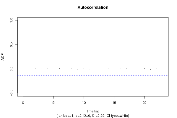
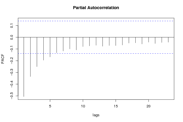
Title produced by software

(Partial) Autocorrelation Function

Date of computation

Tue, 23 Nov 2010 14:56:58 +0000

Cite this page as follows

Statistical Computations at FreeStatistics.org, Office for Research Development and Education, URL https://freestatistics.org/blog/index.php?v=date/2010/Nov/23/t12905241600a3y5dhlf75008f.htm/, Retrieved Sun, 05 May 2024 11:34:27 +0000

Statistical Computations at FreeStatistics.org, Office for Research Development and Education, URL https://freestatistics.org/blog/index.php?pk=99206, Retrieved Sun, 05 May 2024 11:34:27 +0000

QR Codes:

Paste this QR Code to cite your computation.

Original text written by user:

IsPrivate?

No (this computation is public)

User-defined keywords

beursspel test

Estimated Impact

107

Family? (F = Feedback message, R = changed R code, M = changed R Module, P = changed Parameters, D = changed Data)

-       [(Partial) Autocorrelation Function] [TEC autocorrelation] [2010-11-23 14:56:58] [f76239c595e4d455b3b05a43389f68d5] [Current]

Feedback Forum

Post a new message

Dataseries X:

Download CSV

Histogram

Boxplots

0.0077760889499117
3.5527136788005E-15
-0.0077760889498966
1.1546319456102E-14
-0.024497471600388
0.0322735605503
-0.0077760889498966
1.1546319456102E-14
0.0077760889499117
3.5527136788005E-15
3.5527136788005E-15
3.5527136788005E-15
3.5527136788005E-15
-0.0077760889498966
1.1546319456102E-14
1.1546319456102E-14
1.1546319456102E-14
0.0077760889499117
3.5527136788005E-15
0.0023210842142034
0
-0.0077579908108998
3.9523939676656E-14
3.9523939676656E-14
0.0077579908109393
0
0
0
0
-0.0077579908108998
3.9523939676656E-14
3.9523939676656E-14
3.9523939676656E-14
3.9523939676656E-14
3.9523939676656E-14
3.9523939676656E-14
-0.00038948393876082
-4.9293902293357E-14
-4.9293902293357E-14
-4.9293902293357E-14
-4.9293902293357E-14
-0.007036776495049
-2.3980817331903E-14
0.0070367764949757
-4.9293902293357E-14
-4.9293902293357E-14
-0.007036776495049
0.0070367764949757
-4.9293902293357E-14
-4.9293902293357E-14
-4.9293902293357E-14
-0.007036776495049
-2.3980817331903E-14
-2.3980817331903E-14
-2.3980817331903E-14
-2.3980817331903E-14
-2.3980817331903E-14
0.0070367764949757
-0.007036776495049
-2.3980817331903E-14
-2.3980817331903E-14
0.0070367764949757
-0.007036776495049
-2.3980817331903E-14
-2.3980817331903E-14
-2.3980817331903E-14
0.0070367764949757
-4.9293902293357E-14
-4.9293902293357E-14
-0.007036776495049
-2.3980817331903E-14
0.0070367764949757
-4.9293902293357E-14
-4.9293902293357E-14
-4.9293902293357E-14
-4.9293902293357E-14
-4.9293902293357E-14
-4.9293902293357E-14
-0.011361532596849
0.0070671672230582
-0.0070671672231342
0.0070671672230582
-0.0070671672231342
-4.1744385725906E-14
-4.1744385725906E-14
0.00039393343035821
1.2878587085652E-14
-0.0071146545167871
-2.8421709430404E-14
-2.8421709430404E-14
-2.8421709430404E-14
-2.8421709430404E-14
-2.8421709430404E-14
0.0071146545167715
1.2878587085652E-14
1.2878587085652E-14
-0.0071146545167871
-2.8421709430404E-14
-2.8421709430404E-14
-2.8421709430404E-14
0.0071146545167715
1.2878587085652E-14
1.2878587085652E-14
1.2878587085652E-14
1.2878587085652E-14
1.2878587085652E-14
-0.0071146545167871
0.0071146545167715
1.2878587085652E-14
-0.0071146545167871
0.0071146545167715
-0.0071146545167871
0.0071146545167715
1.2878587085652E-14
1.2878587085652E-14
1.2878587085652E-14
1.2878587085652E-14
1.2878587085652E-14
1.2878587085652E-14
1.2878587085652E-14
-0.0071146545167871
-2.8421709430404E-14
0.0071146545167715
1.2878587085652E-14
1.2878587085652E-14
-0.0071146545167871
-2.8421709430404E-14
-2.8421709430404E-14
-2.8421709430404E-14
0.0071146545167715
1.2878587085652E-14
1.2878587085652E-14
1.2878587085652E-14
-0.0071146545167871
-2.8421709430404E-14
-2.8421709430404E-14
-2.8421709430404E-14
-2.8421709430404E-14
-2.8421709430404E-14
-2.8421709430404E-14
-2.8421709430404E-14
-2.8421709430404E-14
-2.8421709430404E-14
-2.8421709430404E-14
0.0071146545167715
1.2878587085652E-14
1.2878587085652E-14
-0.0071146545167871
-2.8421709430404E-14
-2.8421709430404E-14
-2.8421709430404E-14
-2.8421709430404E-14
0.0071146545167715
1.2878587085652E-14
-0.0071146545167871
-2.8421709430404E-14
-2.8421709430404E-14
-2.8421709430404E-14
-2.8421709430404E-14
-2.8421709430404E-14
-2.8421709430404E-14
0.0071146545167715
1.2878587085652E-14
1.2878587085652E-14
1.2878587085652E-14
1.2878587085652E-14
-0.0071146545167871
0.0071146545167715
-0.0071146545167871
-2.8421709430404E-14
-2.8421709430404E-14
0.0071146545167715
-0.0071146545167871
-2.8421709430404E-14
-2.8421709430404E-14
0.015351610285672
-1.1631508098057
1.1241175790765
-7.5495165674511E-15
-7.5495165674511E-15
-7.5495165674511E-15
-7.5495165674511E-15
-7.5495165674511E-15
0.015316704111893
-4.4408920985006E-16
-4.4408920985006E-16
-0.015316704111901
0.015316704111893
-4.4408920985006E-16
-4.4408920985006E-16
-0.015316704111901
-7.5495165674511E-15
-7.5495165674511E-15
-7.5495165674511E-15
0.015316704111893
-4.4408920985006E-16
-0.015316704111901
0.015316704111893
-0.015316704111901
-7.5495165674511E-15

Summary of computational transaction
Raw Input	view raw input (R code)
Raw Output	view raw output of R engine
Computing time	2 seconds
R Server	'Sir Ronald Aylmer Fisher' @ 193.190.124.24

\begin{tabular}{lllllllll}
\hline
Summary of computational transaction \tabularnewline
Raw Input & view raw input (R code)  \tabularnewline
Raw Output & view raw output of R engine  \tabularnewline
Computing time & 2 seconds \tabularnewline
R Server & 'Sir Ronald Aylmer Fisher' @ 193.190.124.24 \tabularnewline
\hline
\end{tabular}
%Source: https://freestatistics.org/blog/index.php?pk=99206&T=0

[TABLE]
[ROW][C]Summary of computational transaction[/C][/ROW]
[ROW][C]Raw Input[/C][C]view raw input (R code) [/C][/ROW]
[ROW][C]Raw Output[/C][C]view raw output of R engine [/C][/ROW]
[ROW][C]Computing time[/C][C]2 seconds[/C][/ROW]
[ROW][C]R Server[/C][C]'Sir Ronald Aylmer Fisher' @ 193.190.124.24[/C][/ROW]
[/TABLE]
Source: https://freestatistics.org/blog/index.php?pk=99206&T=0

Globally Unique Identifier (entire table): ba.freestatistics.org/blog/index.php?pk=99206&T=0

As an alternative you can also use a QR Code:

The GUIDs for individual cells are displayed in the table below:

Summary of computational transaction
Raw Input	view raw input (R code)
Raw Output	view raw output of R engine
Computing time	2 seconds
R Server	'Sir Ronald Aylmer Fisher' @ 193.190.124.24

Autocorrelation Function
Time lag k	ACF(k)	T-STAT	P-value
1	-0.50623	-7.1592	0
2	0.006706	0.0948	0.462272
3	-0.000322	-0.0046	0.498184
4	0.003019	0.0427	0.482993
5	-0.006091	-0.0861	0.465721
6	0.009571	0.1353	0.446236
7	-0.006817	-0.0964	0.461649
8	0.00322	0.0455	0.481863
9	-0.012745	-0.1802	0.42857
10	0.019807	0.2801	0.389842
11	-0.010198	-0.1442	0.442735
12	0.000338	0.0048	0.498096
13	-0.00686	-0.097	0.461405
14	0.007086	0.1002	0.460139
15	-0.003528	-0.0499	0.48013
16	0.003033	0.0429	0.482914
17	0.006596	0.0933	0.462885
18	-0.006708	-0.0949	0.462258
19	-0.006398	-0.0905	0.463995
20	0.013279	0.1878	0.425612
21	-0.013611	-0.1925	0.423776
22	0.01013	0.1433	0.443112
23	-0.003161	-0.0447	0.482192

\begin{tabular}{lllllllll}
\hline
Autocorrelation Function \tabularnewline
Time lag k & ACF(k) & T-STAT & P-value \tabularnewline
1 & -0.50623 & -7.1592 & 0 \tabularnewline
2 & 0.006706 & 0.0948 & 0.462272 \tabularnewline
3 & -0.000322 & -0.0046 & 0.498184 \tabularnewline
4 & 0.003019 & 0.0427 & 0.482993 \tabularnewline
5 & -0.006091 & -0.0861 & 0.465721 \tabularnewline
6 & 0.009571 & 0.1353 & 0.446236 \tabularnewline
7 & -0.006817 & -0.0964 & 0.461649 \tabularnewline
8 & 0.00322 & 0.0455 & 0.481863 \tabularnewline
9 & -0.012745 & -0.1802 & 0.42857 \tabularnewline
10 & 0.019807 & 0.2801 & 0.389842 \tabularnewline
11 & -0.010198 & -0.1442 & 0.442735 \tabularnewline
12 & 0.000338 & 0.0048 & 0.498096 \tabularnewline
13 & -0.00686 & -0.097 & 0.461405 \tabularnewline
14 & 0.007086 & 0.1002 & 0.460139 \tabularnewline
15 & -0.003528 & -0.0499 & 0.48013 \tabularnewline
16 & 0.003033 & 0.0429 & 0.482914 \tabularnewline
17 & 0.006596 & 0.0933 & 0.462885 \tabularnewline
18 & -0.006708 & -0.0949 & 0.462258 \tabularnewline
19 & -0.006398 & -0.0905 & 0.463995 \tabularnewline
20 & 0.013279 & 0.1878 & 0.425612 \tabularnewline
21 & -0.013611 & -0.1925 & 0.423776 \tabularnewline
22 & 0.01013 & 0.1433 & 0.443112 \tabularnewline
23 & -0.003161 & -0.0447 & 0.482192 \tabularnewline
\hline
\end{tabular}
%Source: https://freestatistics.org/blog/index.php?pk=99206&T=1

[TABLE]
[ROW][C]Autocorrelation Function[/C][/ROW]
[ROW][C]Time lag k[/C][C]ACF(k)[/C][C]T-STAT[/C][C]P-value[/C][/ROW]
[ROW][C]1[/C][C]-0.50623[/C][C]-7.1592[/C][C]0[/C][/ROW]
[ROW][C]2[/C][C]0.006706[/C][C]0.0948[/C][C]0.462272[/C][/ROW]
[ROW][C]3[/C][C]-0.000322[/C][C]-0.0046[/C][C]0.498184[/C][/ROW]
[ROW][C]4[/C][C]0.003019[/C][C]0.0427[/C][C]0.482993[/C][/ROW]
[ROW][C]5[/C][C]-0.006091[/C][C]-0.0861[/C][C]0.465721[/C][/ROW]
[ROW][C]6[/C][C]0.009571[/C][C]0.1353[/C][C]0.446236[/C][/ROW]
[ROW][C]7[/C][C]-0.006817[/C][C]-0.0964[/C][C]0.461649[/C][/ROW]
[ROW][C]8[/C][C]0.00322[/C][C]0.0455[/C][C]0.481863[/C][/ROW]
[ROW][C]9[/C][C]-0.012745[/C][C]-0.1802[/C][C]0.42857[/C][/ROW]
[ROW][C]10[/C][C]0.019807[/C][C]0.2801[/C][C]0.389842[/C][/ROW]
[ROW][C]11[/C][C]-0.010198[/C][C]-0.1442[/C][C]0.442735[/C][/ROW]
[ROW][C]12[/C][C]0.000338[/C][C]0.0048[/C][C]0.498096[/C][/ROW]
[ROW][C]13[/C][C]-0.00686[/C][C]-0.097[/C][C]0.461405[/C][/ROW]
[ROW][C]14[/C][C]0.007086[/C][C]0.1002[/C][C]0.460139[/C][/ROW]
[ROW][C]15[/C][C]-0.003528[/C][C]-0.0499[/C][C]0.48013[/C][/ROW]
[ROW][C]16[/C][C]0.003033[/C][C]0.0429[/C][C]0.482914[/C][/ROW]
[ROW][C]17[/C][C]0.006596[/C][C]0.0933[/C][C]0.462885[/C][/ROW]
[ROW][C]18[/C][C]-0.006708[/C][C]-0.0949[/C][C]0.462258[/C][/ROW]
[ROW][C]19[/C][C]-0.006398[/C][C]-0.0905[/C][C]0.463995[/C][/ROW]
[ROW][C]20[/C][C]0.013279[/C][C]0.1878[/C][C]0.425612[/C][/ROW]
[ROW][C]21[/C][C]-0.013611[/C][C]-0.1925[/C][C]0.423776[/C][/ROW]
[ROW][C]22[/C][C]0.01013[/C][C]0.1433[/C][C]0.443112[/C][/ROW]
[ROW][C]23[/C][C]-0.003161[/C][C]-0.0447[/C][C]0.482192[/C][/ROW]
[/TABLE]
Source: https://freestatistics.org/blog/index.php?pk=99206&T=1

Globally Unique Identifier (entire table): ba.freestatistics.org/blog/index.php?pk=99206&T=1

As an alternative you can also use a QR Code:

The GUIDs for individual cells are displayed in the table below:

Autocorrelation Function
Time lag k	ACF(k)	T-STAT	P-value
1	-0.50623	-7.1592	0
2	0.006706	0.0948	0.462272
3	-0.000322	-0.0046	0.498184
4	0.003019	0.0427	0.482993
5	-0.006091	-0.0861	0.465721
6	0.009571	0.1353	0.446236
7	-0.006817	-0.0964	0.461649
8	0.00322	0.0455	0.481863
9	-0.012745	-0.1802	0.42857
10	0.019807	0.2801	0.389842
11	-0.010198	-0.1442	0.442735
12	0.000338	0.0048	0.498096
13	-0.00686	-0.097	0.461405
14	0.007086	0.1002	0.460139
15	-0.003528	-0.0499	0.48013
16	0.003033	0.0429	0.482914
17	0.006596	0.0933	0.462885
18	-0.006708	-0.0949	0.462258
19	-0.006398	-0.0905	0.463995
20	0.013279	0.1878	0.425612
21	-0.013611	-0.1925	0.423776
22	0.01013	0.1433	0.443112
23	-0.003161	-0.0447	0.482192

Partial Autocorrelation Function
Time lag k	PACF(k)	T-STAT	P-value
1	-0.50623	-7.1592	0
2	-0.335555	-4.7455	2e-06
3	-0.250999	-3.5497	0.00024
4	-0.195503	-2.7648	0.003114
5	-0.168353	-2.3809	0.009105
6	-0.13271	-1.8768	0.031001
7	-0.117348	-1.6596	0.049286
8	-0.099763	-1.4109	0.079919
9	-0.10839	-1.5329	0.063445
10	-0.079769	-1.1281	0.130314
11	-0.073789	-1.0435	0.148979
12	-0.068639	-0.9707	0.166435
13	-0.076635	-1.0838	0.139882
14	-0.070658	-0.9993	0.159439
15	-0.071184	-1.0067	0.15765
16	-0.066757	-0.9441	0.173132
17	-0.049722	-0.7032	0.241383
18	-0.047529	-0.6722	0.251127
19	-0.057293	-0.8102	0.20938
20	-0.041981	-0.5937	0.276694
21	-0.053246	-0.753	0.226164
22	-0.044661	-0.6316	0.264182
23	-0.042157	-0.5962	0.275861

\begin{tabular}{lllllllll}
\hline
Partial Autocorrelation Function \tabularnewline
Time lag k & PACF(k) & T-STAT & P-value \tabularnewline
1 & -0.50623 & -7.1592 & 0 \tabularnewline
2 & -0.335555 & -4.7455 & 2e-06 \tabularnewline
3 & -0.250999 & -3.5497 & 0.00024 \tabularnewline
4 & -0.195503 & -2.7648 & 0.003114 \tabularnewline
5 & -0.168353 & -2.3809 & 0.009105 \tabularnewline
6 & -0.13271 & -1.8768 & 0.031001 \tabularnewline
7 & -0.117348 & -1.6596 & 0.049286 \tabularnewline
8 & -0.099763 & -1.4109 & 0.079919 \tabularnewline
9 & -0.10839 & -1.5329 & 0.063445 \tabularnewline
10 & -0.079769 & -1.1281 & 0.130314 \tabularnewline
11 & -0.073789 & -1.0435 & 0.148979 \tabularnewline
12 & -0.068639 & -0.9707 & 0.166435 \tabularnewline
13 & -0.076635 & -1.0838 & 0.139882 \tabularnewline
14 & -0.070658 & -0.9993 & 0.159439 \tabularnewline
15 & -0.071184 & -1.0067 & 0.15765 \tabularnewline
16 & -0.066757 & -0.9441 & 0.173132 \tabularnewline
17 & -0.049722 & -0.7032 & 0.241383 \tabularnewline
18 & -0.047529 & -0.6722 & 0.251127 \tabularnewline
19 & -0.057293 & -0.8102 & 0.20938 \tabularnewline
20 & -0.041981 & -0.5937 & 0.276694 \tabularnewline
21 & -0.053246 & -0.753 & 0.226164 \tabularnewline
22 & -0.044661 & -0.6316 & 0.264182 \tabularnewline
23 & -0.042157 & -0.5962 & 0.275861 \tabularnewline
\hline
\end{tabular}
%Source: https://freestatistics.org/blog/index.php?pk=99206&T=2

[TABLE]
[ROW][C]Partial Autocorrelation Function[/C][/ROW]
[ROW][C]Time lag k[/C][C]PACF(k)[/C][C]T-STAT[/C][C]P-value[/C][/ROW]
[ROW][C]1[/C][C]-0.50623[/C][C]-7.1592[/C][C]0[/C][/ROW]
[ROW][C]2[/C][C]-0.335555[/C][C]-4.7455[/C][C]2e-06[/C][/ROW]
[ROW][C]3[/C][C]-0.250999[/C][C]-3.5497[/C][C]0.00024[/C][/ROW]
[ROW][C]4[/C][C]-0.195503[/C][C]-2.7648[/C][C]0.003114[/C][/ROW]
[ROW][C]5[/C][C]-0.168353[/C][C]-2.3809[/C][C]0.009105[/C][/ROW]
[ROW][C]6[/C][C]-0.13271[/C][C]-1.8768[/C][C]0.031001[/C][/ROW]
[ROW][C]7[/C][C]-0.117348[/C][C]-1.6596[/C][C]0.049286[/C][/ROW]
[ROW][C]8[/C][C]-0.099763[/C][C]-1.4109[/C][C]0.079919[/C][/ROW]
[ROW][C]9[/C][C]-0.10839[/C][C]-1.5329[/C][C]0.063445[/C][/ROW]
[ROW][C]10[/C][C]-0.079769[/C][C]-1.1281[/C][C]0.130314[/C][/ROW]
[ROW][C]11[/C][C]-0.073789[/C][C]-1.0435[/C][C]0.148979[/C][/ROW]
[ROW][C]12[/C][C]-0.068639[/C][C]-0.9707[/C][C]0.166435[/C][/ROW]
[ROW][C]13[/C][C]-0.076635[/C][C]-1.0838[/C][C]0.139882[/C][/ROW]
[ROW][C]14[/C][C]-0.070658[/C][C]-0.9993[/C][C]0.159439[/C][/ROW]
[ROW][C]15[/C][C]-0.071184[/C][C]-1.0067[/C][C]0.15765[/C][/ROW]
[ROW][C]16[/C][C]-0.066757[/C][C]-0.9441[/C][C]0.173132[/C][/ROW]
[ROW][C]17[/C][C]-0.049722[/C][C]-0.7032[/C][C]0.241383[/C][/ROW]
[ROW][C]18[/C][C]-0.047529[/C][C]-0.6722[/C][C]0.251127[/C][/ROW]
[ROW][C]19[/C][C]-0.057293[/C][C]-0.8102[/C][C]0.20938[/C][/ROW]
[ROW][C]20[/C][C]-0.041981[/C][C]-0.5937[/C][C]0.276694[/C][/ROW]
[ROW][C]21[/C][C]-0.053246[/C][C]-0.753[/C][C]0.226164[/C][/ROW]
[ROW][C]22[/C][C]-0.044661[/C][C]-0.6316[/C][C]0.264182[/C][/ROW]
[ROW][C]23[/C][C]-0.042157[/C][C]-0.5962[/C][C]0.275861[/C][/ROW]
[/TABLE]
Source: https://freestatistics.org/blog/index.php?pk=99206&T=2

Globally Unique Identifier (entire table): ba.freestatistics.org/blog/index.php?pk=99206&T=2

As an alternative you can also use a QR Code:

The GUIDs for individual cells are displayed in the table below:

Partial Autocorrelation Function
Time lag k	PACF(k)	T-STAT	P-value
1	-0.50623	-7.1592	0
2	-0.335555	-4.7455	2e-06
3	-0.250999	-3.5497	0.00024
4	-0.195503	-2.7648	0.003114
5	-0.168353	-2.3809	0.009105
6	-0.13271	-1.8768	0.031001
7	-0.117348	-1.6596	0.049286
8	-0.099763	-1.4109	0.079919
9	-0.10839	-1.5329	0.063445
10	-0.079769	-1.1281	0.130314
11	-0.073789	-1.0435	0.148979
12	-0.068639	-0.9707	0.166435
13	-0.076635	-1.0838	0.139882
14	-0.070658	-0.9993	0.159439
15	-0.071184	-1.0067	0.15765
16	-0.066757	-0.9441	0.173132
17	-0.049722	-0.7032	0.241383
18	-0.047529	-0.6722	0.251127
19	-0.057293	-0.8102	0.20938
20	-0.041981	-0.5937	0.276694
21	-0.053246	-0.753	0.226164
22	-0.044661	-0.6316	0.264182
23	-0.042157	-0.5962	0.275861

Figure 1

PNG link

Postscript link

PDF link

Figure 2

PNG link

Postscript link

PDF link

Parameters (Session):

par1 = Default ; par2 = 1 ; par3 = 0 ; par4 = 0 ; par5 = 12 ; par6 = White Noise ; par7 = 0.95 ;

Parameters (R input):

par1 = Default ; par2 = 1 ; par3 = 0 ; par4 = 0 ; par5 = 12 ; par6 = White Noise ; par7 = 0.95 ;

R code (references can be found in the software module):

if (par1 == 'Default') {
par1 = 10*log10(length(x))
} else {
par1 <- as.numeric(par1)
}
par2 <- as.numeric(par2)
par3 <- as.numeric(par3)
par4 <- as.numeric(par4)
par5 <- as.numeric(par5)
if (par6 == 'White Noise') par6 <- 'white' else par6 <- 'ma'
par7 <- as.numeric(par7)
if (par2 == 0) {
x <- log(x)
} else {
x <- (x ^ par2 - 1) / par2
}
if (par3 > 0) x <- diff(x,lag=1,difference=par3)
if (par4 > 0) x <- diff(x,lag=par5,difference=par4)
bitmap(file='pic1.png')
racf <- acf(x, par1, main='Autocorrelation', xlab='time lag', ylab='ACF', ci.type=par6, ci=par7, sub=paste('(lambda=',par2,', d=',par3,', D=',par4,', CI=', par7, ', CI type=',par6,')',sep=''))
dev.off()
bitmap(file='pic2.png')
rpacf <- pacf(x,par1,main='Partial Autocorrelation',xlab='lags',ylab='PACF')
dev.off()
(myacf <- c(racf$acf))
(mypacf <- c(rpacf$acf))
lengthx <- length(x)
sqrtn <- sqrt(lengthx)
load(file='createtable')
a<-table.start()
a<-table.row.start(a)
a<-table.element(a,'Autocorrelation Function',4,TRUE)
a<-table.row.end(a)
a<-table.row.start(a)
a<-table.element(a,'Time lag k',header=TRUE)
a<-table.element(a,hyperlink('basics.htm','ACF(k)','click here for more information about the Autocorrelation Function'),header=TRUE)
a<-table.element(a,'T-STAT',header=TRUE)
a<-table.element(a,'P-value',header=TRUE)
a<-table.row.end(a)
for (i in 2:(par1+1)) {
a<-table.row.start(a)
a<-table.element(a,i-1,header=TRUE)
a<-table.element(a,round(myacf[i],6))
mytstat <- myacf[i]*sqrtn
a<-table.element(a,round(mytstat,4))
a<-table.element(a,round(1-pt(abs(mytstat),lengthx),6))
a<-table.row.end(a)
}
a<-table.end(a)
table.save(a,file='mytable.tab')
a<-table.start()
a<-table.row.start(a)
a<-table.element(a,'Partial Autocorrelation Function',4,TRUE)
a<-table.row.end(a)
a<-table.row.start(a)
a<-table.element(a,'Time lag k',header=TRUE)
a<-table.element(a,hyperlink('basics.htm','PACF(k)','click here for more information about the Partial Autocorrelation Function'),header=TRUE)
a<-table.element(a,'T-STAT',header=TRUE)
a<-table.element(a,'P-value',header=TRUE)
a<-table.row.end(a)
for (i in 1:par1) {
a<-table.row.start(a)
a<-table.element(a,i,header=TRUE)
a<-table.element(a,round(mypacf[i],6))
mytstat <- mypacf[i]*sqrtn
a<-table.element(a,round(mytstat,4))
a<-table.element(a,round(1-pt(abs(mytstat),lengthx),6))
a<-table.row.end(a)
}
a<-table.end(a)
table.save(a,file='mytable1.tab')

Free Statistics

Description of Statistical Computation

Tree of Dependent Computations

Dataset

Tables (Output of Computation)

Figures (Output of Computation)

Input Parameters & R Code