Free Statistics
of Irreproducible Research!
Description of Statistical Computation | |||||||||||||||||||||||||||||||||||||||||||||||||||||||||||||
|---|---|---|---|---|---|---|---|---|---|---|---|---|---|---|---|---|---|---|---|---|---|---|---|---|---|---|---|---|---|---|---|---|---|---|---|---|---|---|---|---|---|---|---|---|---|---|---|---|---|---|---|---|---|---|---|---|---|---|---|---|---|
| Author's title | |||||||||||||||||||||||||||||||||||||||||||||||||||||||||||||
| Author | *The author of this computation has been verified* | ||||||||||||||||||||||||||||||||||||||||||||||||||||||||||||
| R Software Module | rwasp_linear_regression.wasp | ||||||||||||||||||||||||||||||||||||||||||||||||||||||||||||
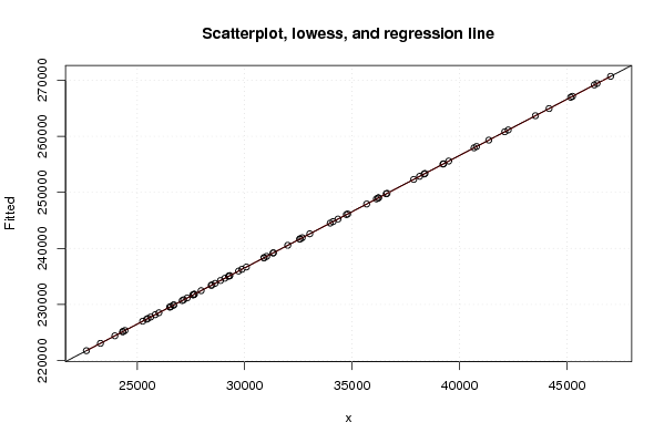
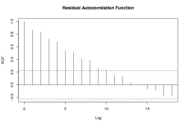
| Title produced by software | Linear Regression Graphical Model Validation | ||||||||||||||||||||||||||||||||||||||||||||||||||||||||||||
| Date of computation | Wed, 24 Nov 2010 18:27:12 +0000 | ||||||||||||||||||||||||||||||||||||||||||||||||||||||||||||
| Cite this page as follows | Statistical Computations at FreeStatistics.org, Office for Research Development and Education, URL https://freestatistics.org/blog/index.php?v=date/2010/Nov/24/t12906235895vfd8esoey2ml6g.htm/, Retrieved Fri, 03 May 2024 10:31:40 +0000 | ||||||||||||||||||||||||||||||||||||||||||||||||||||||||||||
| Statistical Computations at FreeStatistics.org, Office for Research Development and Education, URL https://freestatistics.org/blog/index.php?pk=100497, Retrieved Fri, 03 May 2024 10:31:40 +0000 | |||||||||||||||||||||||||||||||||||||||||||||||||||||||||||||
| QR Codes: | |||||||||||||||||||||||||||||||||||||||||||||||||||||||||||||
|
| |||||||||||||||||||||||||||||||||||||||||||||||||||||||||||||
| Original text written by user: | |||||||||||||||||||||||||||||||||||||||||||||||||||||||||||||
| IsPrivate? | No (this computation is public) | ||||||||||||||||||||||||||||||||||||||||||||||||||||||||||||
| User-defined keywords | |||||||||||||||||||||||||||||||||||||||||||||||||||||||||||||
| Estimated Impact | 166 | ||||||||||||||||||||||||||||||||||||||||||||||||||||||||||||
Tree of Dependent Computations | |||||||||||||||||||||||||||||||||||||||||||||||||||||||||||||
| Family? (F = Feedback message, R = changed R code, M = changed R Module, P = changed Parameters, D = changed Data) | |||||||||||||||||||||||||||||||||||||||||||||||||||||||||||||
| - [Linear Regression Graphical Model Validation] [] [2010-11-24 18:27:12] [b7dd4adfab743bef2d672ff51f950617] [Current] - D [Linear Regression Graphical Model Validation] [Paper Statistiek] [2010-12-27 11:07:48] [b2f924a86c4fbfa8afa1027f3839f526] - PD [Linear Regression Graphical Model Validation] [] [2010-12-27 12:55:37] [b2f924a86c4fbfa8afa1027f3839f526] - PD [Linear Regression Graphical Model Validation] [Simple Linear Reg...] [2010-12-27 16:45:21] [fd57ceeb2f72ef497e1390930b11fced] - [Linear Regression Graphical Model Validation] [] [2010-12-27 20:22:09] [b2f924a86c4fbfa8afa1027f3839f526] | |||||||||||||||||||||||||||||||||||||||||||||||||||||||||||||
| Feedback Forum | |||||||||||||||||||||||||||||||||||||||||||||||||||||||||||||
Post a new message | |||||||||||||||||||||||||||||||||||||||||||||||||||||||||||||
Dataset | |||||||||||||||||||||||||||||||||||||||||||||||||||||||||||||
| Dataseries X: | |||||||||||||||||||||||||||||||||||||||||||||||||||||||||||||
22631 23956 23284 24334 24319 25252 24427 25434 25496 26681 25624 26706 25834 26513 26005 27158 26521 27652 26566 27597 27605 28621 27090 27652 28440 29076 27326 28477 29303 29301 27972 29247 29871 30079 28873 30897 30902 31321 29714 32006 31338 32562 31024 32678 33031 34115 32574 33984 34795 35680 34342 36136 36226 36226 34736 36588 45176 38351 36629 38146 39232 39257 37869 38394 40681 40797 39500 41366 42270 43536 42109 45262 46406 46275 44171 47037 | |||||||||||||||||||||||||||||||||||||||||||||||||||||||||||||
| Dataseries Y: | |||||||||||||||||||||||||||||||||||||||||||||||||||||||||||||
186448 190530 194207 190855 200779 204428 207617 212071 214239 215883 223484 221529 225247 226699 231406 232324 237192 236727 240698 240688 245283 243556 247826 245798 250479 249216 251896 247616 249994 246552 248771 247551 249745 245742 249019 245841 248771 244723 246878 246014 248496 244351 248016 246509 249426 247840 251035 250161 254278 250801 253985 249174 251287 247947 249992 243805 255812 250417 253033 248705 253950 251484 251093 245996 252721 248019 250464 245571 252690 250183 253639 254436 265280 268705 270643 271480 | |||||||||||||||||||||||||||||||||||||||||||||||||||||||||||||
Tables (Output of Computation) | |||||||||||||||||||||||||||||||||||||||||||||||||||||||||||||
| |||||||||||||||||||||||||||||||||||||||||||||||||||||||||||||
Figures (Output of Computation) | |||||||||||||||||||||||||||||||||||||||||||||||||||||||||||||
Input Parameters & R Code | |||||||||||||||||||||||||||||||||||||||||||||||||||||||||||||
| Parameters (Session): | |||||||||||||||||||||||||||||||||||||||||||||||||||||||||||||
| par1 = 0 ; | |||||||||||||||||||||||||||||||||||||||||||||||||||||||||||||
| Parameters (R input): | |||||||||||||||||||||||||||||||||||||||||||||||||||||||||||||
| par1 = 0 ; | |||||||||||||||||||||||||||||||||||||||||||||||||||||||||||||
| R code (references can be found in the software module): | |||||||||||||||||||||||||||||||||||||||||||||||||||||||||||||
par1 <- as.numeric(par1) | |||||||||||||||||||||||||||||||||||||||||||||||||||||||||||||